Use these links to easily see the "What's New" pages for previous releases of Mechanical. Use the first link to return to this "2021 R2 What's New" page.

2021 R2 What's New (You are here)
2021 R1 What's New

Helpful Links

These are for your convenience. Some require Ansys Customer Portal login credentials.

Graphics

Importing Image for Model Overlay

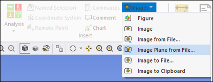
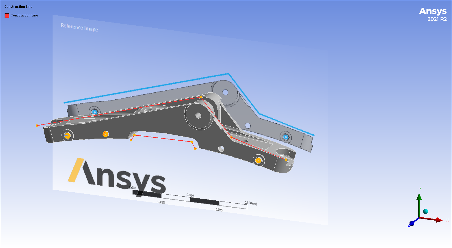
You can now place logos on your model (shown below), specify a background, set up physical rulers to help measure deformations, incorporate image planes into custom ACT extensions, and other creative uses of imported images by using the new Image Plane from File option of the Images drop-down menu. The feature enables you to import an image into Mechanical and place it on or around your model based on the XY-plane of the selected coordinate system. The feature originated as an option from the Construction Line object to overlay and accurately sketch line segments, but has been expanded to allow more diverse uses.

Want to learn more? If you are on Windows, go to the documentation for this topic.
(Requires internet access and will open in a new browser window. Not for Linux platforms.)

Flexible Probe Display

In previous releases, the application deleted probe labels whenever you made a change to the Deformation Scale Factor. Now, by turning on the new Move Probe Labels with Deformation Scale Factor preference, Mechanical no longer deletes probes when you change the scale factor. The probes are “flexible” and move with the deformed mesh.

Want to learn more? If you are on Windows, go to the documentation for this topic.
(Requires internet access and will open in a new browser window. Not for Linux platforms.)

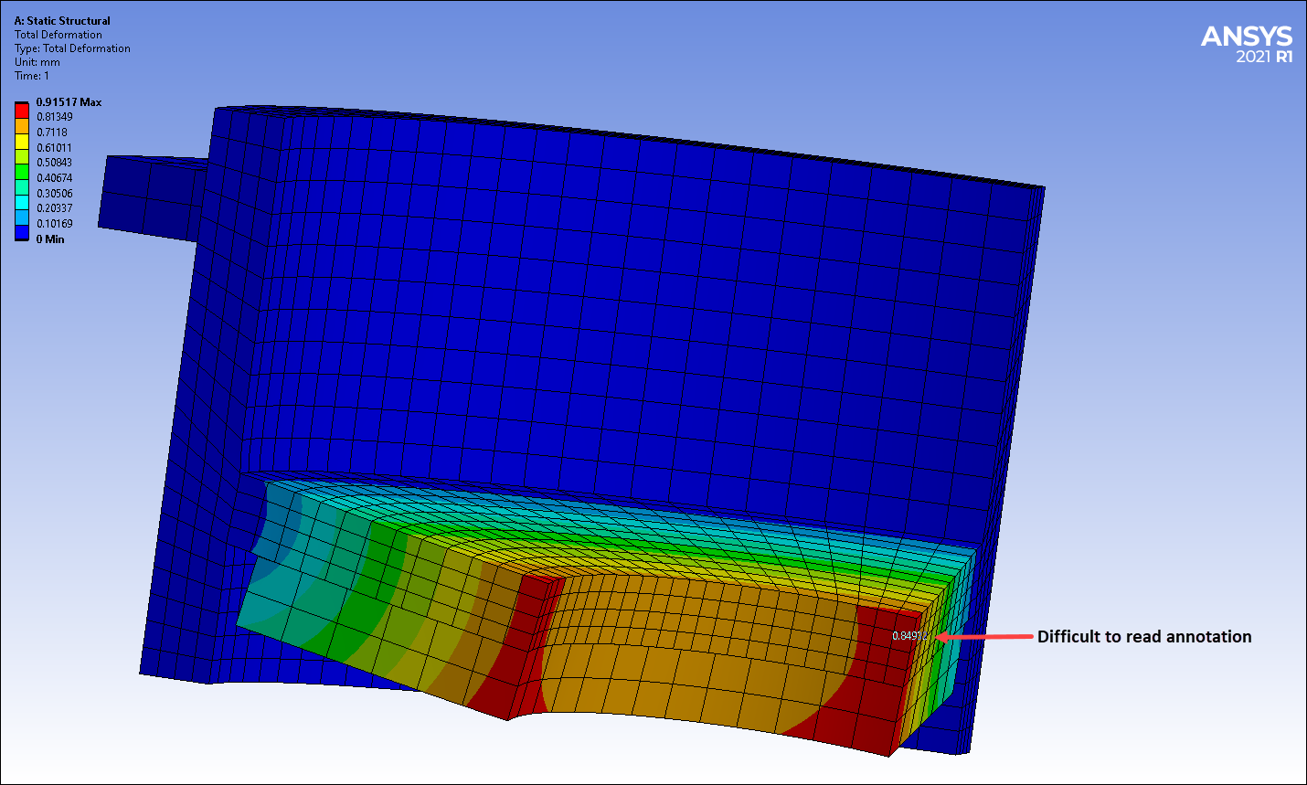
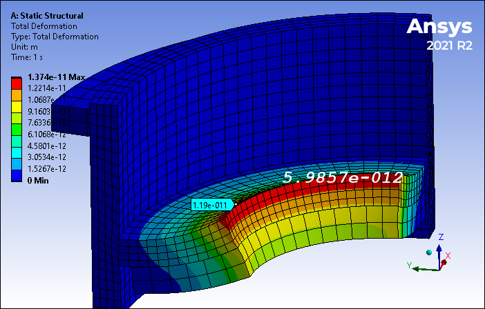
Probe Annotation Display

When defining probe annotations, the new Probe Font (Windows Only) preference enables you to change the default setting of the displayed font type (Arial, Times Roman, etc.), size, style (bold or italic), and color. Previously, as shown in the first image below, the color of the annotation changed based on the background color. This sometimes resulted in a blurred display. When you set the Probe Font (Windows Only) preference, the display is much clearer and easier to be read, as you can see from the second image.

Want to learn more? If you are on Windows, go to the documentation for this topic.
(Requires internet access and will open in a new browser window. Not for Linux platforms.)

External Model

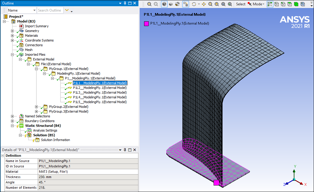
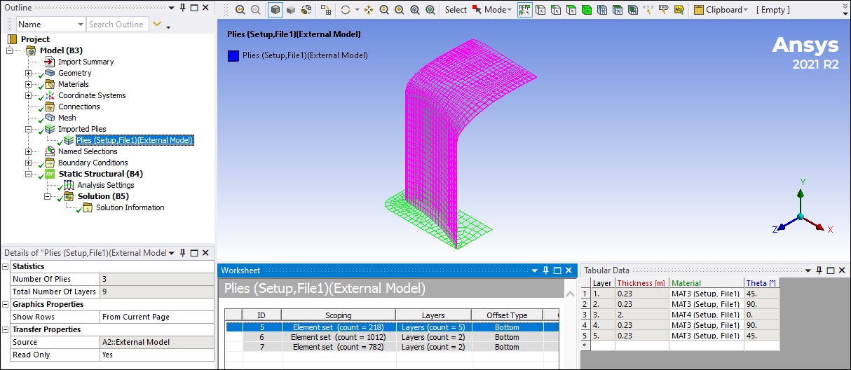
Imported Composite Plies

Previously, as shown in the first image below, when you imported composite ply data from External Model, the application presented the imported data as a cascading hierarchy of child objects, each including imported data. This made models with many plies difficult to manage. Now, as shown in the second image, the application presents the imported data in the Worksheet and in the Tabular Data window using a singular object.

Want to learn more? If you are on Windows, go to the documentation for this topic.
(Requires internet access and will open in a new browser window. Not for Linux platforms.)

Mesh

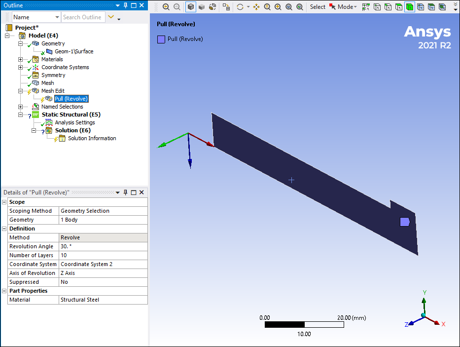
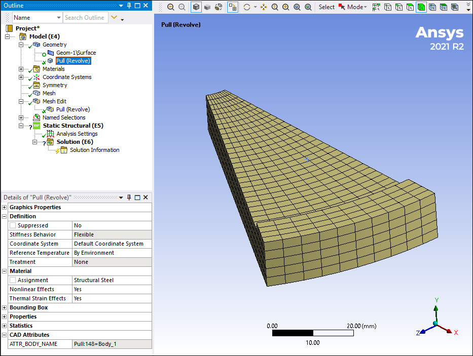
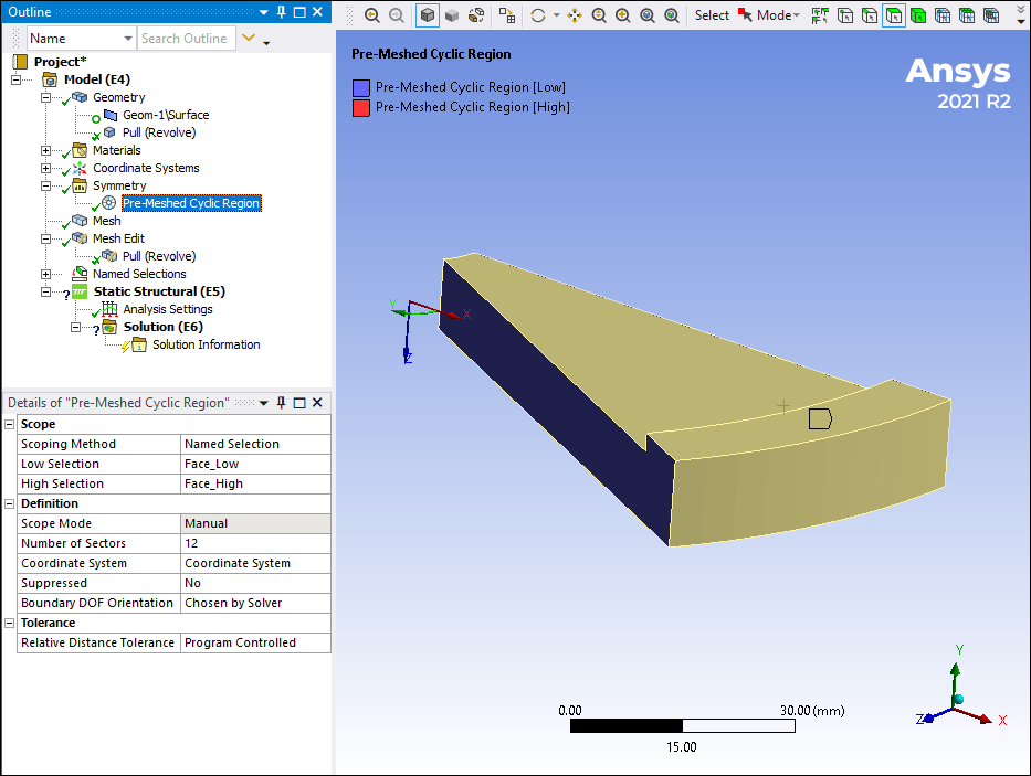
Mesh Extrusions Using Pull

Mechanical lets you create an extruded mesh from an existing meshed surface or volume using the new Pull mesh feature. Its options include Extrude, Revolve, and Surface Coating. With these you can create new meshed bodies that can be used in your analyses. In the example shown here, you can create a 3D sector from a surface body using the Revolve option. This new body can then be used to perform a cyclic symmetry analysis.

Want to learn more? If you are on Windows, go to the documentation for this topic.
(Requires internet access and will open in a new browser window. Not for Linux platforms.)

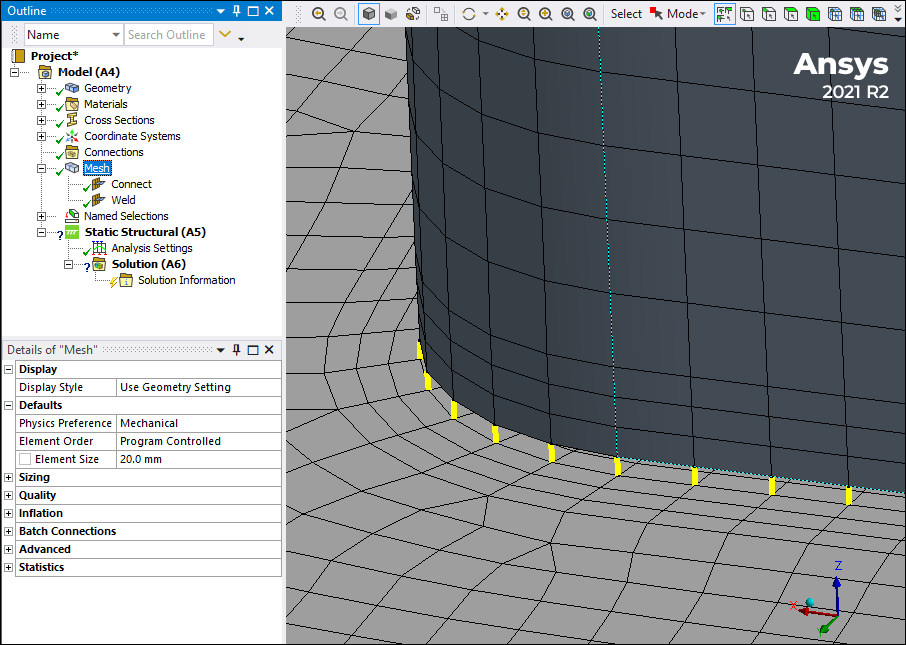
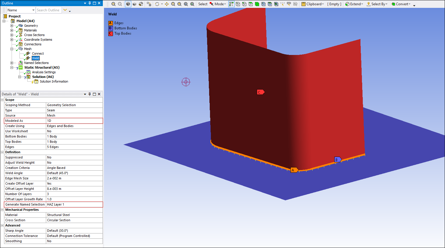
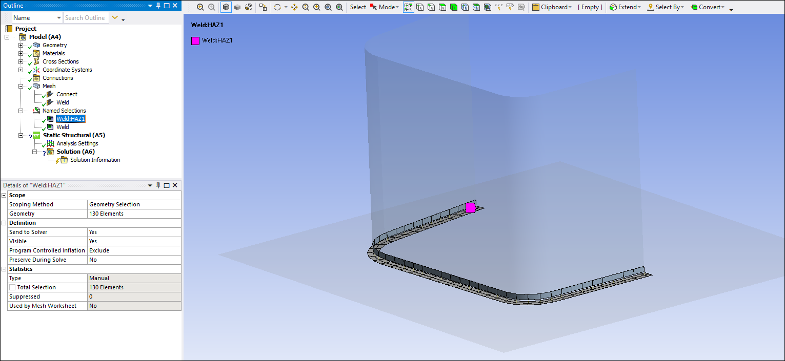
Weld Meshing

The automatic weld meshing tools have been enhanced for 1D weld mesh, Named Selection creation on HAZ (Heat Affected Zone) layers, and error handling for complex models with the Worksheet view.

Want to learn more? If you are on Windows, go to the documentation for this topic.
(Requires internet access and will open in a new browser window. Not for Linux platforms.)

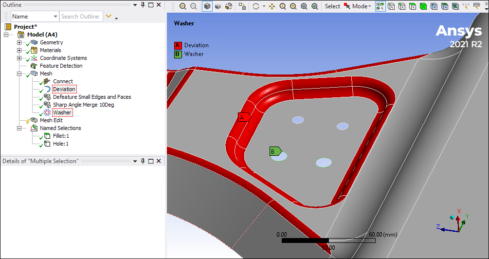
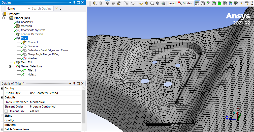
Feature Detection and Treatment

Within the weld meshing workflow, Mechanical now enables you to automatically detect and apply mesh treatments to fillets and holes in sheet bodies. The Fillet mesh treatment is a Deviation control allowing multiple ways to control the number of elements in the primary curvature direction of the fillet. The 2D hole mesh treatment is a Washer control, and it enables insertion of 1-3 layers of quad elements around the hole.

Want to learn more? If you are on Windows, go to the Deviation documentation or the Washer documentation.
(Requires internet access and will open in a new browser window. Not for Linux platforms.)

Connections

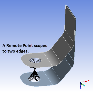
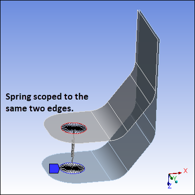
Display of Remote Point Connections

A new display feature, Remote Point Connections, is now available from the Style group on the Display tab and supports a number of remote boundary conditions. In previous releases, you could only do a visual check of connection lines between an underlying geometry and a remote point. Now, remote boundary conditions can make use of remote points that are either specifically defined or created internally by the application. As a result, in addition to remote points, you can view connection lines for the following:

Beam Connections
Bearing
Joints
Moment
Point Mass

Remote Displacement
Remote Force
Spring
Spot Weld
Thermal Point Mass

Want to learn more? If you are on Windows, go to the documentation for this topic.
(Requires internet access and will open in a new browser window. Not for Linux platforms.)

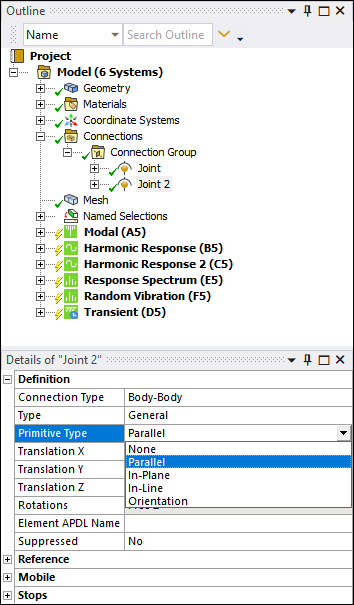
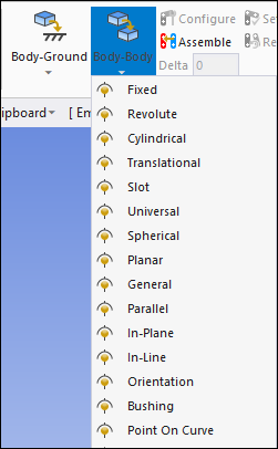
General Joint

Now, when you insert a General Joint, a new property: Primitive Type, enables you to predefine the joint's degrees of freedom as either Parallel, In-Plane, In-Line, or Orientation. In addition to being available from the Primitive Type property of the General Joint, the options are also available from the Joint drop-down menus on the Connections tab so that you can insert the preferred type directly.

Want to learn more? If you are on Windows, go to the documentation for this topic.
(Requires internet access and will open in a new browser window. Not for Linux platforms.)

Analysis

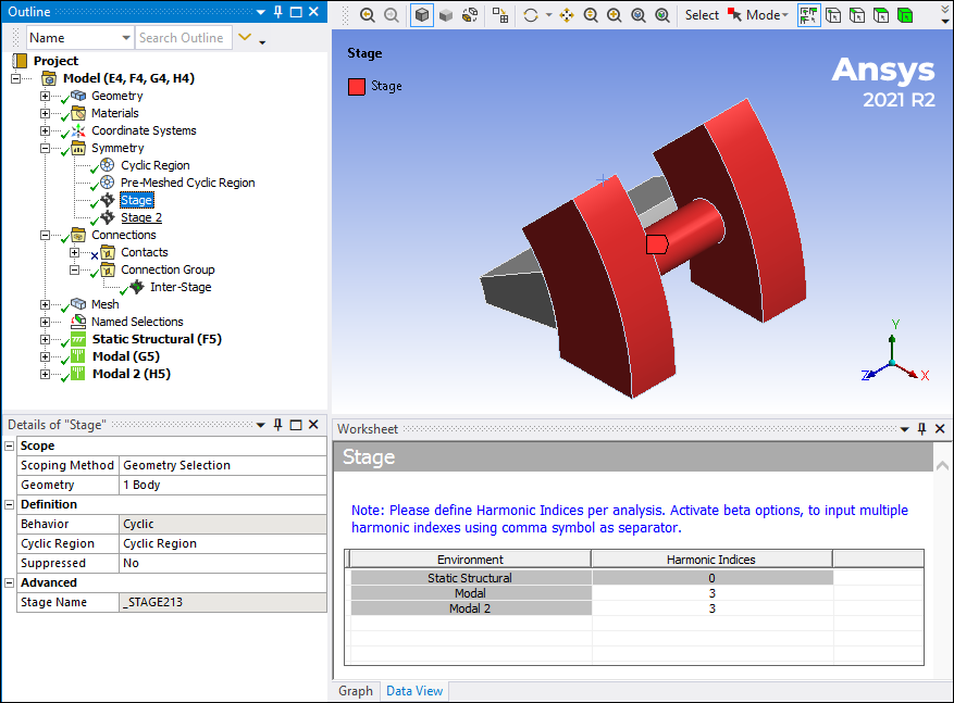
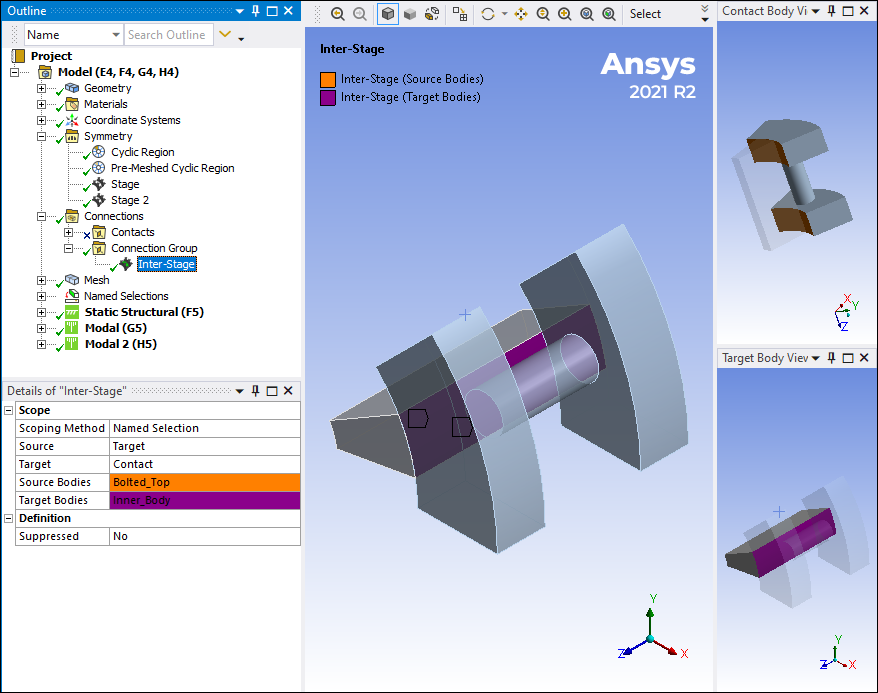
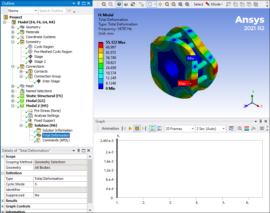
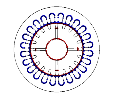
Multistage Cyclic Symmetry

With this new innovative technology, you can connect multiple cyclic symmetry structures with different sector counts for analysis, making possible accurate and efficient simulation of rotationally periodic structures such as gears and turbomachinery assemblies.

Want to learn more? If you are on Windows, go to the documentation for this topic.
(Requires internet access and will open in a new browser window. Not for Linux platforms.)

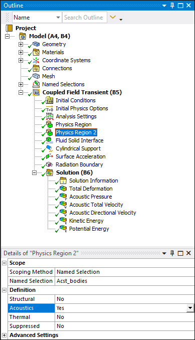
Coupled Field Acoustics

Coupled Field Transient analysis supports simulation with standalone Acoustics physics and coupled Structural-Acoustics physics. Coupled Field Modal and Coupled Field Harmonic analysis can couple Acoustics physics in addition to Piezoelectric coupling or can be used for standalone Acoustics physics simulation.

Want to learn more? If you are on Windows, go to the documentation for this topic.
(Requires internet access and will open in a new browser window. Not for Linux platforms.)

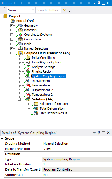
Coupled Field Static and Coupled Field Transient

With this release, the Coupled Field Static and Coupled Field Transient analyses support use of the System Coupling Region object. This allows the coupling of structural quantities (force, displacement) and thermal quantities (temperature, heat flow, heat transfer coefficient, near-wall temperature) to integrate a Mechanical analysis with System Coupling.

Want to learn more? If you are on Windows, go to the documentation for this topic.
(Requires internet access and will open in a new browser window. Not for Linux platforms.)

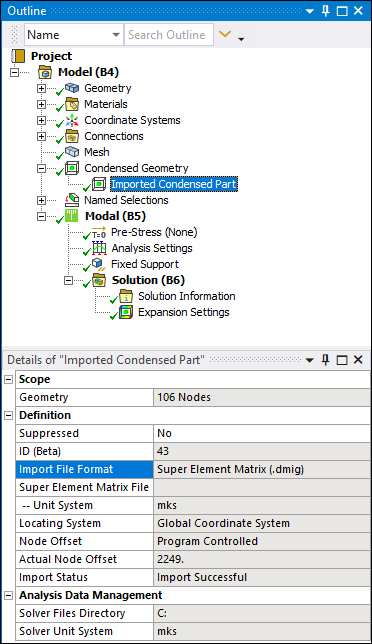
Imported Condensed Part

At 2021 R2, the Imported Condensed Part feature lets you import condensed parts using the Generation Pass Output (.sub) and Super Element Matrix (.dmig) file formats.

Want to learn more? If you are on Windows, go to the documentation for this topic.
(Requires internet access and will open in a new browser window. Not for Linux platforms.)

Fracture

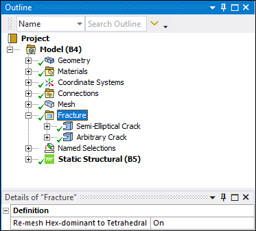
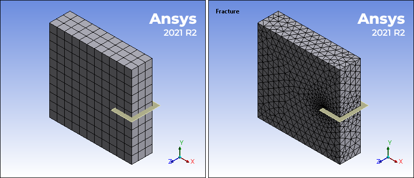
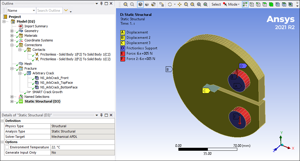
Fracture Object

The Fracture object has a new property, Re-mesh Hex-dominant to Tetrahedral. Turning this property On will automatically re-mesh a hex-dominant base mesh, on the solid body of Arbitrary Crack (including imported mesh) and Semi-Elliptical Crack objects, to a tetrahedral mesh. This is especially useful for an imported hex-dominant mesh, which can then be re-meshed to tetrahedrons before being used to generate the initial crack mesh for the fracture parameters calculation and SMART Crack Growth.

Want to learn more? If you are on Windows, go to the documentation for this topic.
(Requires internet access and will open in a new browser window. Not for Linux platforms.)

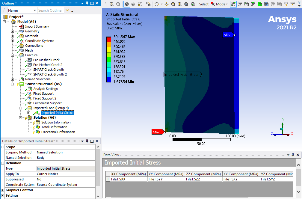
SMART Crack Growth

The SMART Crack Growth feature:

Is no longer limited by the type of contact defined in the model.
Now supports Initial Stress as an Imported Load type.

Want to learn more? If you are on Windows, go to the documentation for this topic.
(Requires internet access and will open in a new browser window. Not for Linux platforms.)

Loading and Support Conditions

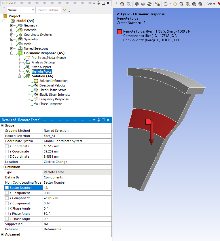
Non-Cyclic Loading for Full Harmonic Response Analyses

The Non-Cyclic Loading Type property now supports Sector Number entries, either an individual sector entry or multiple sectors using Tabular Data.

Want to learn more? If you are on Windows, go to the documentation for this topic.
(Requires internet access and will open in a new browser window. Not for Linux platforms.)

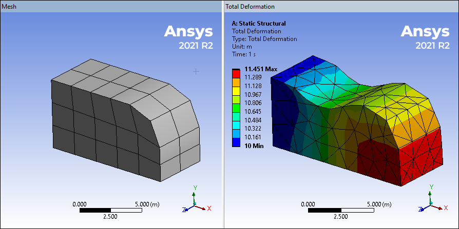
Nonlinear Adaptive Region

You can now scope the Nonlinear Adaptive Region to a body that is meshed with hexahedral-dominant elements. During the solution process, this mesh gets converted to a tetrahedral mesh after the criterion for the re-mesh of the Nonlinear Adaptive Region is met.

Want to learn more? If you are on Windows, go to the documentation for this topic.
(Requires internet access and will open in a new browser window. Not for Linux platforms.)

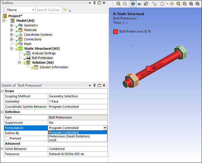
Bolt Pretension Formulation

The Bolt Pretension loading condition has a new property: Formulation. Currently, the Bolt Pretension load uses element PRETS179 to simulate the pretension. This element does not account for rotation of the bolt and as a result, the analysis may not converge if the bolt is undergoing rotation. Using the new Formulation property, Joint, instructs the application to use element MPC184. This element updates the bolt loading direction as the bolt undergoes rotation and therefore helps the solution converge.

Want to learn more? If you are on Windows, go to the documentation for this topic.
(Requires internet access and will open in a new browser window. Not for Linux platforms.)

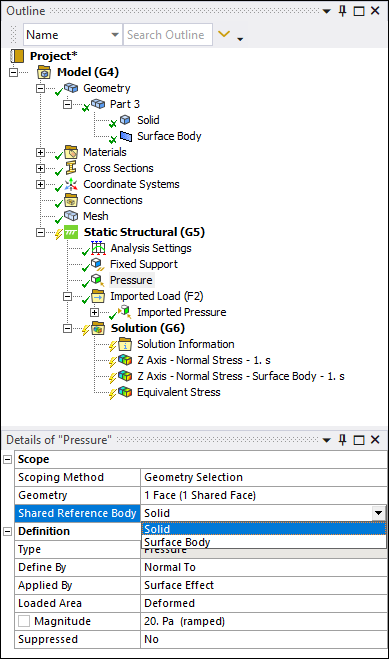
Loading Condition Scoping for Shared Topology

For the following loading conditions, a new Shared Reference Body property is available when two bodies share topology. This property provides a drop-down list of the bodies that share scoping. You select one of the bodies, either solid or surface, to specify a desired direction, thickness, or surface property for the loading condition:

Pressure/Imported Pressure
Hydrostatic Pressure
Convection/Imported Convection Coefficient
Radiation

Want to learn more? If you are on Windows, go to the documentation for this topic.
(Requires internet access and will open in a new browser window. Not for Linux platforms.)

Solution

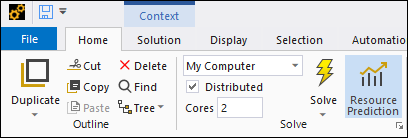
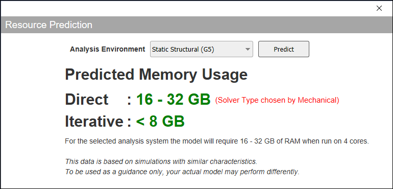
Resource Prediction

The new Resource Prediction option (Home Tab/Solve Group) calculates an estimate of the required computing resources needed to perform a solution for the analysis environment you specify. This feature is supported for a standalone Static Structural analysis and for Modal analyses.

Want to learn more? If you are on Windows, go to the documentation for this topic.
(Requires internet access and will open in a new browser window. Not for Linux platforms.)

Explicit Dynamics

LS-DYNA

The following enhancements have been made at Release 2021 R2 for the LS-DYNA Workbench system:

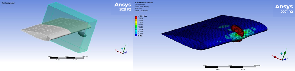
The Structured ALE LS-DYNA solver is now available in the LS-DYNA system in Workbench. This analysis is useful as an alternative to SPH for bird strike, or for modeling an underwater blast.

Want to learn more? If you are on Windows, go to the documentation for this topic.
(Requires internet access and will open in a new browser window. Not for Linux platforms.)
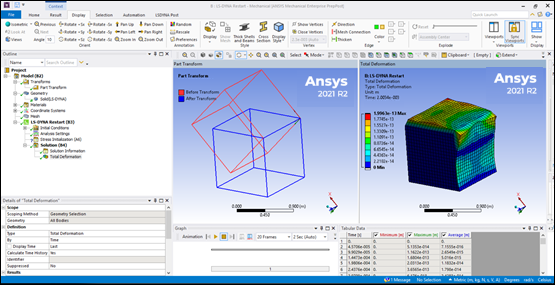
The restart capability has been improved. The restart simulation can be defined in a different model than the primary calculation. Another restart enhancement is that you can now add additional geometric bodies to a solved analysis.

Want to learn more? If you are on Windows, go to the documentation for this topic.
(Requires internet access and will open in a new browser window. Not for Linux platforms.)
Preloading can now be done using implicit features of the LS-DYNA solver as an alternative to using the Mechanical APDL solver, to maximize compatibility between explicit and preloading calculations.
LS-DYNA supports the mortar types of contact. Mortar contact is the preferred contact algorithm for implicit calculations.

Want to learn more? If you are on Windows, go to the documentation for this topic.
(Requires internet access and will open in a new browser window. Not for Linux platforms.)
The LS-DYNA system is now available on the Linux platform.

Results and Post Processing

Result Scale Menu

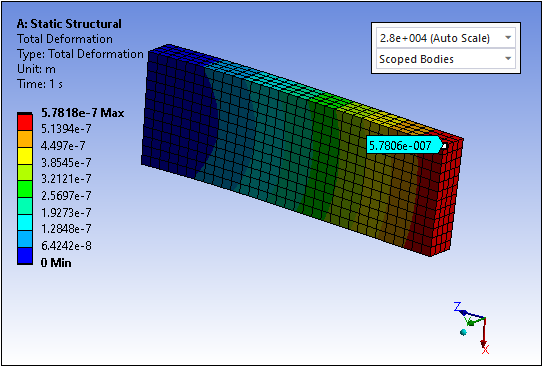
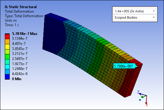
In previous releases, if you wanted to customize the scale factor, you entered a value in the field and it was treated as a multiplier. If you clicked on a result at a different time or re-evaluated the result at a different time, the scale multiplier would change based on the corresponding deformation.

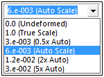
Now, when you specify a positive number as a multiplier, you affect the True Scale (actual deformation) and the application does not change the value when you re-evaluate the result or select another result.

In addition, Automatic Scale multiplier entries are still available but are now set by entering a negative number. This new scheme of positive and negative values distinguishes the difference between True Scale and Auto Scale.

Want to learn more? If you are on Windows, go to the documentation for this topic.
(Requires internet access and will open in a new browser window. Not for Linux platforms.)

Scripting

Python Code Object

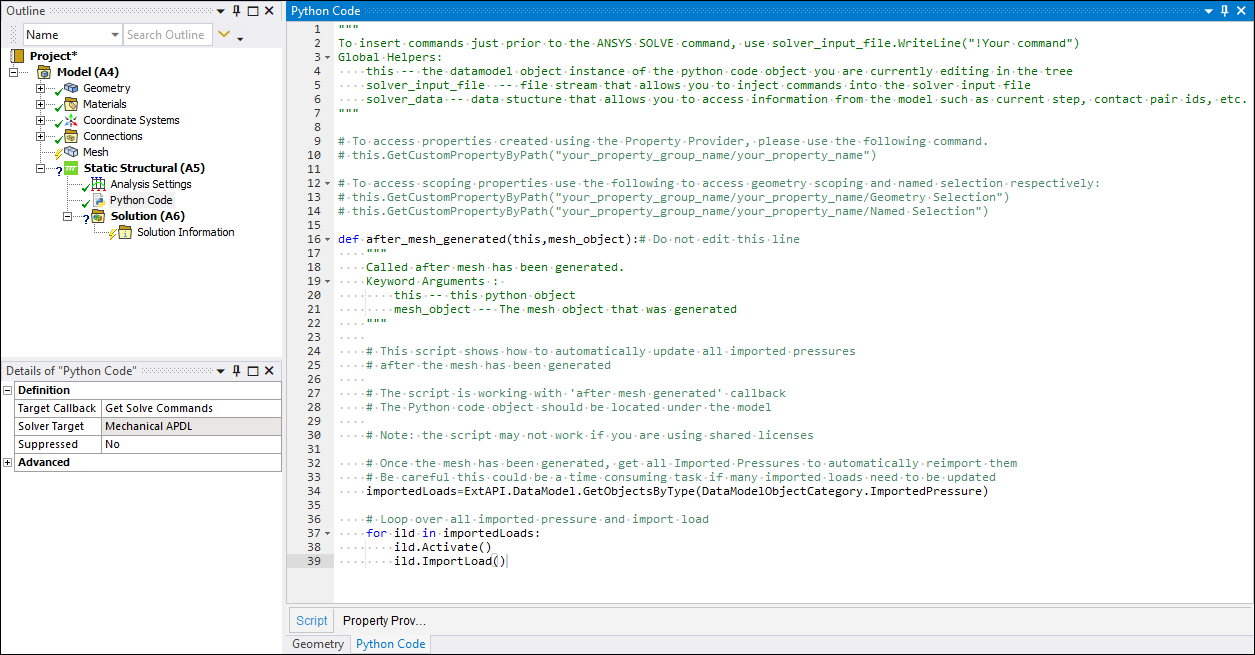
Mechanical now offers an object for Python scripting that supports the execution of Python code. In this way, you can inject Mechanical APDL commands into the solver input and run Python code during key events to drive the simulation. This feature supports the addition of custom properties to the details for user input.

Want to learn more? If you are on Windows, go to the documentation for this topic.
(Requires internet access and will open in a new browser window. Not for Linux platforms.)

Structural Optimization

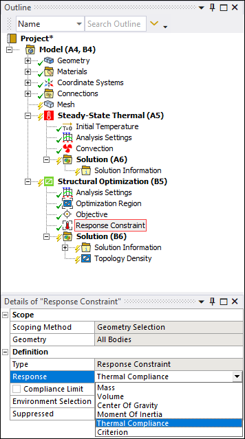
Thermal Compliance

The Topology Optimization Level-Set Based and Shape Optimization methods now enable you to specify Thermal Compliance as a Response Constraint as well as the Response Type of the Objective.

Want to learn more? If you are on Windows, go to the documentation for this topic.
(Requires internet access and will open in a new browser window. Not for Linux platforms.)

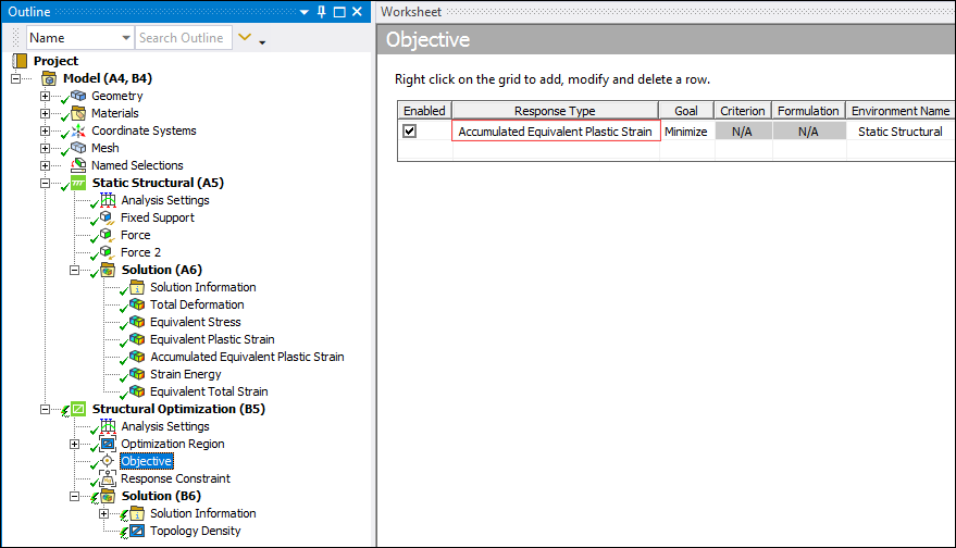
Nonlinear Structural Analyses

You can now use the Shape Optimization method with a Structural analysis that includes plastic behavior. Along with this capability, there is a new Accumulated Plastic Strain option available for the Response Type setting of the Objective. This option is also the new default.

Want to learn more? If you are on Windows, go to the documentation for this topic.
(Requires internet access and will open in a new browser window. Not for Linux platforms.)

Ansys Motion

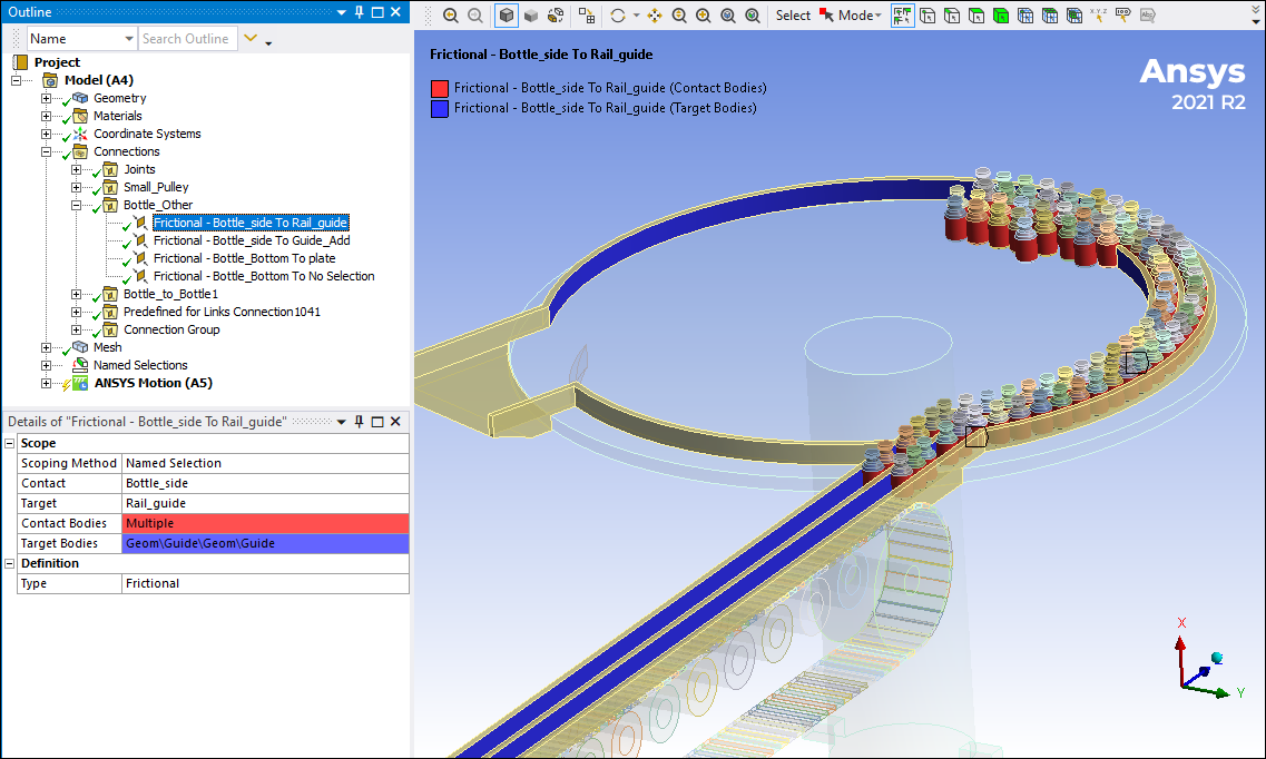
Contact Enhancements

Ansys Motion now supports contact regions defined between multiple bodies, improving usability for large models:

Want to learn more? If you are on Windows, go to the documentation for this topic.
(Requires internet access and will open in a new browser window. Not for Linux platforms.)

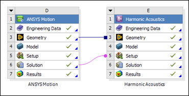
Acoustic Coupling

A Harmonic Acoustics system can now be linked to an upstream Ansys Motion system to perform one-way vibroacoustic analysis to capture the acoustic behavior of a vibrating structure. Structural velocities from Ansys Motion are converted from the time domain to the frequency domain before being mapped on the acoustic domain mesh.

Want to learn more? If you are on Windows, go to the documentation for this topic.
(Requires internet access and will open in a new browser window. Not for Linux platforms.)

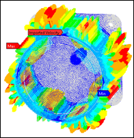
Electromagnetic Coupling

You can now import result files from Maxwell simulations, transferring electromagnetic forces for application to an electric motor at specific rotational speeds. Imported forces are displayed in the Graphics pane.

Want to learn more? If you are on Windows, go to the documentation for this topic.
(Requires internet access and will open in a new browser window. Not for Linux platforms.)

Additive Manufacturing

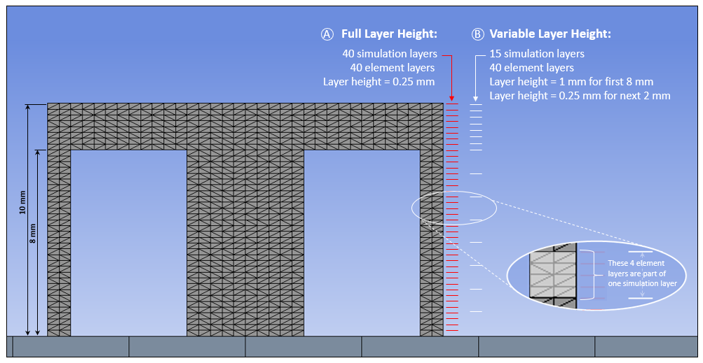
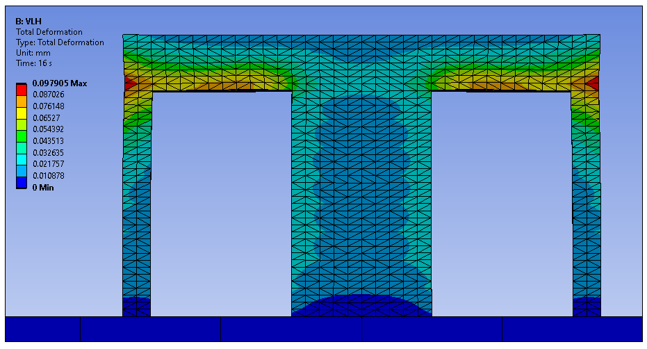
Workbench Additive

Using the new variable layer height feature, you can now vary the simulation's layer height to build with smaller layers in areas of interest, and larger layers in other areas of the part. You can capture fine details in a simulation without greatly increasing, and sometimes even reducing, the overall simulation time by reducing the number of super-layer steps that need to be solved.

Want to learn more? If you are on Windows, go to the documentation for this topic.
(Requires internet access and will open in a new browser window. Not for Linux platforms.)