As ACCS is completely integrated within ANSYS Workbench, one simply needs to run Workbench to have access to it.
For step-by-step tutorials, please refer to the Workshops section.
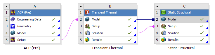
A typical Workbench ACCS workflow for composite structures looks as follows:
Fig. 3.1 Typical cure simulation workflow for composites in Workbench.
The material properties are defined in the Engineering Data module. A shell model is generated in DesignModeler or in SpaceClaim or in any other CAD tool, then it is worked out in ACP (Pre) module to build a solid finite element model of the composite structure that will be transferred to the “Transient Thermal” module where the temperature distribution will be computed throughout the cure cycle for every element as well as the degree of cure, the state of the material, the glass transition temperature and the instantaneous heat of reaction. The temperature distribution is then transferred to the “Static Structural” module where the distortions will be computed using the previously computed temperature and the material properties.
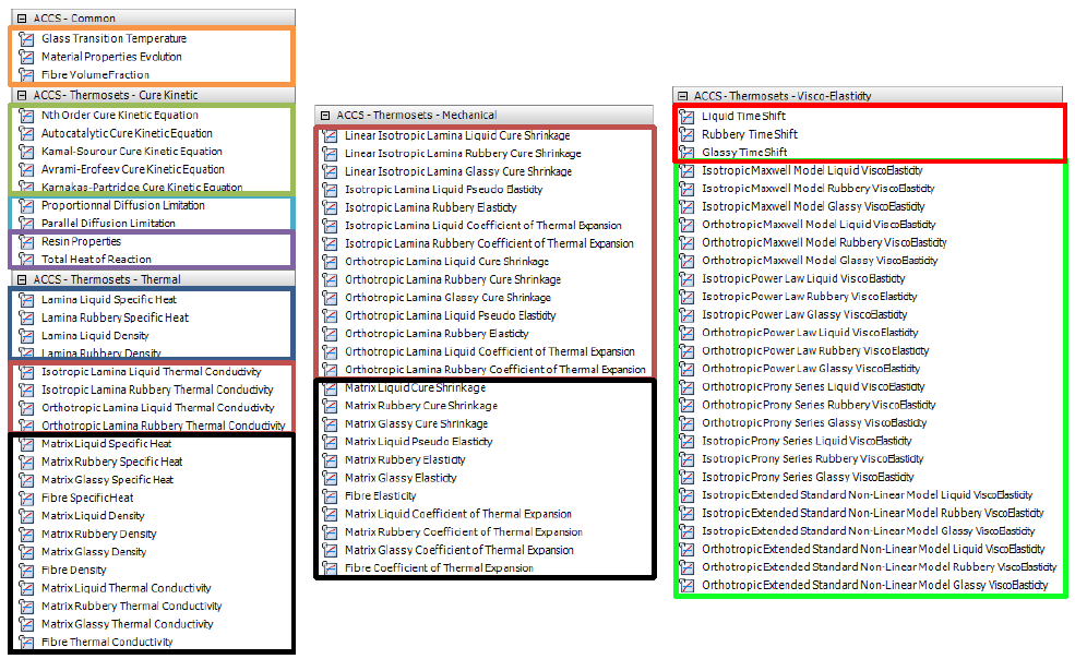
The first task in the modeling of the cure process with ACCS is to correctly define the material properties. In the list of Materials (Fig. 3.2), the basic material properties that the user should start with are the Thermoset - Cure Kinetics Model [first five Properties ended with “Equation”]. The Resin properties, Total Heat of Reaction and the ACCS Common properties will be included automatically. The user can then include a diffusion limitation formulation (Proportional Diffusion Limitation or Parallel Diffusion Limitation). Now the user must choose one of the two ways to define the ply material. The first one is defining the ply material using separate fiber and matrix properties, which in this case all the properties enclosed by a black rectangle must be included (adding one will include the other relevant properties). The second way is to define the ply material using homogenized lamina properties. In this case the Isotropic or Orthotropic properties must be included (adding one will also include the other relevant properties). All the first four properties of the “ACCS-Thermoset-Thermal” list will also be included automatically. Optionally, the user may want to include visco-elastic effects. To do so, the user can include one of the available models in its Isotropic or Orthotropic formulation (in light green). Adding one will include the other relevant properties. Including the “Liquid Time Shift”, “Rubbery Time Shift” and “Glassy Time Shift” properties will allow to take into effect temperature and/or degree of cure time shifts.
Fig. 3.2 List of material properties specific for Thermosets showed in the Engineering Data
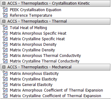
Fig. 3.3 List of material properties specific for Thermoplastics showed in the Engineering Data
For the PEEK Crystallization model, the user has to introduce all of the thermoplastics properties and all of the fibre properties. When the PEEK Crystallization Model is introduced in the Engineering Data, all the rest of the thermoplastic material properties (Thermal and Mechanical) will be automatically included into the material definition. For more detail about this crystallization model, please refer to its section in the theory documentation.
Note
The automatic inclusion of properties is only available for Engineering Data cells connected to an “ACP (Pre)” module, an ANSYS thermal module or an ANSYS structural module.
Warning
When opening in ANSYS 2022 R1 a project which was created with an earlier release of ACCS, the material properties must be updated. Simply click on the button .
Note
If in Engineering Data, the materials were introduced using the fibre/matrix formulation, the user can add equivalent glassy properties to fix some issues. Simply click on the button .
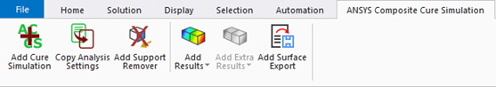
The ACCS solution is also integrated within Mechanical and is therefore available in the Transient Thermal and Static Structural analysis systems in the form of an additional tab in the ribbon as show in the figure below.
Fig. 3.4 ACCS features in the Mechanical menu ribbon.
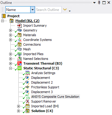
Adding ACCS to the analysis invokes the ANSYS solver with chemical cure and cure shrinkage routines for materials with defined cure kinetics properties within the Engineering Data module. Once in Workbench Mechanical the user can initiate ACCS by clicking on the “Add Cure Simulation” button as shown in the figures below for the Transient Thermal and Static Structural modules.
Fig. 3.5 Initiating ACCS from the toolbar adds an “ANSYS Composite Cure Simulation” item to the current analysis.
When performing a Full Cure Simulation, the button “Copy Analysis Settings” allows the user to copy relevant analysis settings between two analyses easy and fast.
Fig. 3.6 This pop up window appears when selecting the “copy Analysis Settings” feature.
The lamination process usually involves the placing of composite layers over a mold. After the curing cycle is finished, the part is taken off the mold. Is in this phase of the process where the most relevant permanent deformations occur since the part is without the form constrictions. To simulate that step, ACCS has a boundary condition called “Support Remover” which delete every node that is scoped to it from it predefined displacement constraint. It is important to remark that the support remover is only needed for frictionless supports because you cannot enable/disable it per load step as other supports do.
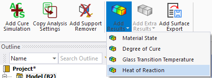
Including the ACCS feature into the analysis opens the possibility to add cure simulation specific post-processing options like Material State, Degree of Cure, Glass Transition Temperature and Cure Shrinkage in all cartesian directions. These options can be found by selecting the “Add Results” and the “Add Extra Results” buttons, as shown in the following image:
Fig. 3.8 Results available during both the Thermal and Mechanical analyses.
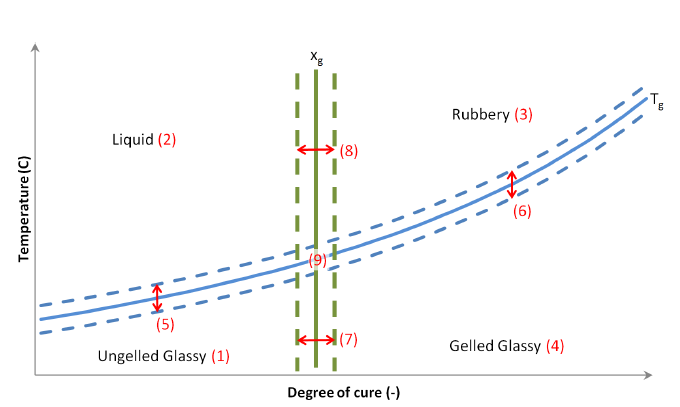
There are two main transitions that can be distinguished during the curing process of a thermosetting resin. The first one is gelation and the second one is vitrification occurring when the material Tg reaches the cure temperature
Fig. 3.9 Plot of an empirical curve (blue) and a simplified curve (red dots) used by ACCS to describe the different material states.
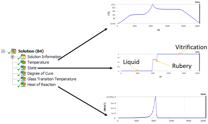
This result shows the develope of the curing reaction in the material domain. See Fig. 4.1 to see a the dependence of the degree of cure and the temperature in time.
The Heat of Reaction is shown in the Thermoset domain and the plot shows the evolution of it in the time window.
Once the model is solved, the results can be reviewed by clicking on them. Here in the example, an exothermic reaction can be seen in the temperature profile. In many cases, the exothermic reaction a risk to the process. Excessive heat can cause inhomogeneous cure (check the Degree of Cure result) and can damage the structural materials (mainly the resin itself, but also polymeric sandwich cores; or heat-sensitive fibers, such as natural fibers), as well as the auxiliary materials (e.g. the vacuum bag).
Fig. 3.10 Solution plots example. Exotherms and material states can be post processed from thermal simulation.
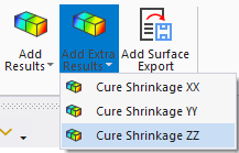
Fig. 3.11 Extra results only available during the Mechanical analysis.
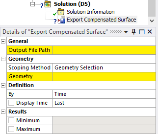
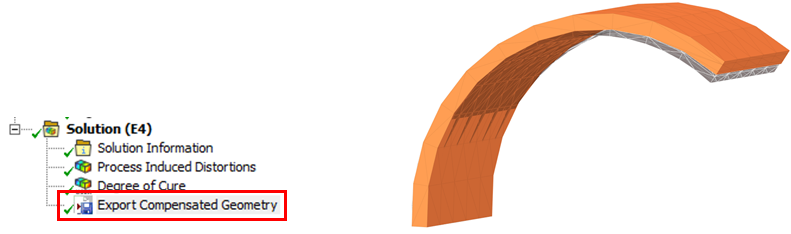
The export compensated geometry button adds an object which automatically compensates the process induced distortions for the selected faces. The process induced distortions (deformations) of the structural simulation are inverted and added to the nominal geometry. The compensated geometry can be exported as STL, RSO or point cloud. The options of the support remover are:
Output File Path: the file path where the file will be saved
Scoping Method and Geometry: the geometrical entities which will be exported
Fig. 3.12 Options of the compensated surface export item.
Fig. 3.13 Compensated geometry (orange) and nominal shape (grey).
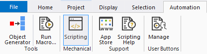
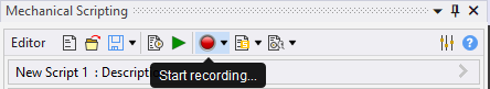
The automatization suite of Mechanical also supports the scripting of the ACCS extension. The example below shows how the ACCS extension and module can be loaded into the scripting environment.
Once loaded, the ACCS module can be used to activate the curing simulation, control the properties, add a support remover, add results plots etc.
This example shows how a full cure simulation with a transient thermal and structural analysis can be defined via scripting. The first script (wbjn) adds the material to the WB project and the analysis systems, the second script (Python) is for Mechanical to add, configure, run, and post-process the cure simulation within Mechanical.
This example shows how a fast cure simulation with a three-step structural analysis can be defined via scripting. The first script (wbjn) adds the material to the WB project and the analysis system, the second script (Python) is for Mechanical to add, configure, run, and post-process the cure simulation within Mechanical. The cure cycle is defined by the manufacturer recommended cure-cycle (heat rate, and dwell times).
This example shows how a fast cure simulation with a three-step structural analysis can be defined via scripting. The first script (wbjn) adds the material to the WB project and the analysis system, the second script (Python) is for Mechanical to add, configure, run, and post-process the cure simulation within Mechanical. The cure cycle is defined by the temperature versus time curve.
1# encoding: utf-8 2 3Reset() 4 5importos 6importre 7 8directory=os.path.dirname(os.path.abspath(__file__)) 9cdb=os.path.join(directory,"C-shape.cdb")10script=os.path.join(directory,"test_scripting_fast_Tvst.py")111213importACCS_scripting141516# Instantiating the project interface17ACCS_proj=ACCS_scripting.Project()18192021EngD_sys=GetTemplate(TemplateName="EngData").CreateSystem()22EngD_EngD=EngD_sys.GetContainer(ComponentName="Engineering Data")23forminEngD_EngD.GetMaterials():24m.Delete()25EngD_fav=EngData.LoadFavoriteItems()26EngD_lib=EngData.OpenLibrary(Name="Cure Simulation",Source="ACCS_Library.xml")27AS4=EngD_EngD.ImportMaterial(Name="UD epoxy prepreg",Source="ACCS_Library.xml")28AS4.SetAsDefaultSolidForModel()29AS4.SetAsDefaultFluidForModel()30EngD_engd=EngD_sys.GetComponent(Name="Engineering Data")313233FEM_sys=GetTemplate(TemplateName="External Model").CreateSystem(Position="Below",RelativeTo=EngD_sys)34FEM_sys.GetContainer(ComponentName="Setup").AddDataFile(FilePath=cdb)35FEM_setup=FEM_sys.GetComponent(Name="Setup")36FEM_setup.Update(AllDependencies=True)37383940MaterialReleases=ACCS_proj.CheckMaterial()41ifMaterialReleases!=None:42print("Materials need to be updated")43ACCS_proj.UpgradeMaterial()444546ACCS_proj.HomogeneizeMaterial()47484950St_tpl=GetTemplate(TemplateName="Static Structural",Solver="ANSYS")51Fast_Tvst_sys=St_tpl.CreateSystem(Position="Right",RelativeTo=FEM_sys)52Fast_Tvst_sys.DisplayText="Fast T vs t - Static Structural"53Fast_Tvst_engd=Fast_Tvst_sys.GetComponent(Name="Engineering Data")54Fast_Tvst_model=Fast_Tvst_sys.GetComponent(Name="Model")55Fast_Tvst_setup=Fast_Tvst_sys.GetContainer(ComponentName="Setup")5657Fast_Tvst_engd.ReplaceWithShare(TargetSystem=Fast_Tvst_sys,ComponentToShare=EngD_engd,SourceSystem=EngD_sys)58FEM_setup.TransferData(TargetComponent=Fast_Tvst_model)596061Fast_Tvst_model.Update(AllDependencies=True)626364Fast_Tvst_setup.Edit()65Fast_Tvst_setup.SendCommand(Command="WB.AppletList.Applet('DSApplet').App.Script.doToolsRunMacro(\""+re.escape(script)+"\")")
1# encoding: utf-8 2 3Reset() 4 5importos 6importre 7 8directory=os.path.dirname(os.path.abspath(__file__)) 9cdb=os.path.join(directory,"C-shape.cdb")10script=os.path.join(directory,"test_scripting_fast_Tvst.py")111213importACCS_scripting141516# Instantiating the project interface17ACCS_proj=ACCS_scripting.Project()18192021EngD_sys=GetTemplate(TemplateName="EngData").CreateSystem()22EngD_EngD=EngD_sys.GetContainer(ComponentName="Engineering Data")23forminEngD_EngD.GetMaterials():24m.Delete()25EngD_fav=EngData.LoadFavoriteItems()26EngD_lib=EngData.OpenLibrary(Name="Cure Simulation",Source="ACCS_Library.xml")27AS4=EngD_EngD.ImportMaterial(Name="UD epoxy prepreg",Source="ACCS_Library.xml")28AS4.SetAsDefaultSolidForModel()29AS4.SetAsDefaultFluidForModel()30EngD_engd=EngD_sys.GetComponent(Name="Engineering Data")313233FEM_sys=GetTemplate(TemplateName="External Model").CreateSystem(Position="Below",RelativeTo=EngD_sys)34FEM_sys.GetContainer(ComponentName="Setup").AddDataFile(FilePath=cdb)35FEM_setup=FEM_sys.GetComponent(Name="Setup")36FEM_setup.Update(AllDependencies=True)37383940MaterialReleases=ACCS_proj.CheckMaterial()41ifMaterialReleases!=None:42print("Materials need to be updated")43ACCS_proj.UpgradeMaterial()444546ACCS_proj.HomogeneizeMaterial()47484950St_tpl=GetTemplate(TemplateName="Static Structural",Solver="ANSYS")51Fast_Tvst_sys=St_tpl.CreateSystem(Position="Right",RelativeTo=FEM_sys)52Fast_Tvst_sys.DisplayText="Fast T vs t - Static Structural"53Fast_Tvst_engd=Fast_Tvst_sys.GetComponent(Name="Engineering Data")54Fast_Tvst_model=Fast_Tvst_sys.GetComponent(Name="Model")55Fast_Tvst_setup=Fast_Tvst_sys.GetContainer(ComponentName="Setup")5657Fast_Tvst_engd.ReplaceWithShare(TargetSystem=Fast_Tvst_sys,ComponentToShare=EngD_engd,SourceSystem=EngD_sys)58FEM_setup.TransferData(TargetComponent=Fast_Tvst_model)596061Fast_Tvst_model.Update(AllDependencies=True)626364Fast_Tvst_setup.Edit()65Fast_Tvst_setup.SendCommand(Command="WB.AppletList.Applet('DSApplet').App.Script.doToolsRunMacro(\""+re.escape(script)+"\")")
 .
. .
.
 button as shown in the figures below for the Transient Thermal and Static Structural modules.
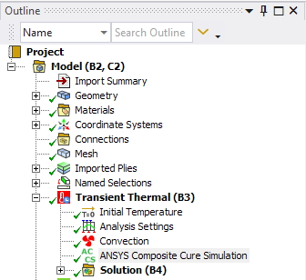
 allows the user to copy relevant analysis settings between two analyses easy and fast.
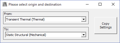
 which delete every node that is scoped to it from it predefined displacement constraint. It is important to remark that the support remover is only needed for frictionless supports because you cannot enable/disable it per load step as other supports do.
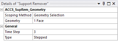
 adds an object which automatically compensates the process induced distortions for the selected faces. The process induced distortions (deformations) of the structural simulation are inverted and added to the nominal geometry. The compensated geometry can be exported as STL, RSO or point cloud. The options of the support remover are: