4. Best Practices
Some suggestions on how to model properly the cure cycle are given in the following sections:
4.1. How to Define an Autoclave Cycle
4.1.1. Number of Steps
To determine the proper number of steps, one must understand first the curing cycle. The thermal portion in a classic autoclave cycle for a 170 °C curing thermoset epoxy part is shown schematically in Fig. 4.1. It contains two ramps and two isothermal holds. The first ramp and isothermal hold, usually in the range of 115–130 °C, is used to allow the resin to flow (bleed) and volatiles to escape. For simplicity, a constant film coefficient of 5 J/msup:`2 K can be considered for the air convection in the autoclave. The viscosity curve of the semi-solid resin matrix melts on heating and experiences a dramatic drop in viscosity. The second ramp and hold is the polymerization portion of the cure cycle. During this portion, the resin viscosity initially drops slightly due to the application of additional heat and then rises dramatically as the kinetics of the resin start the cross-linking process. The resin gels into a solid and the cross-linking process continues during the second isothermal hold, usually at 170–190 °C for epoxy resin systems. The resin is held at this cure temperature for normally 4–6 h, allowing time for the cross-linking process to be completed. It should be noted that as the industry has moved towards net resin content systems, the use of the first isothermal hold which allows time for resin bleeding has been eliminated by many manufacturers resulting in a straight ramp-up to the curing temperature as illustrated in Fig. 4.1.
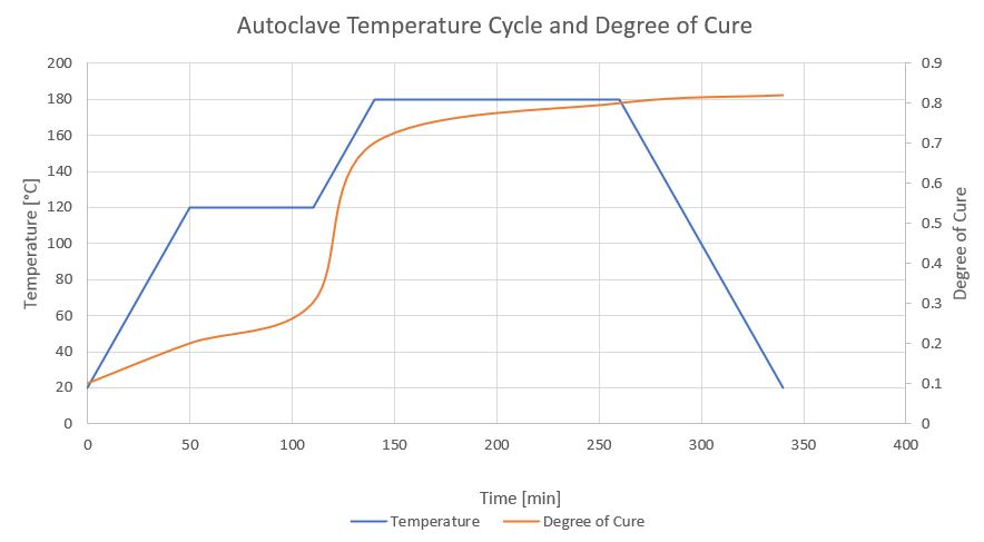
Fig. 4.1 Scheme of a typical autoclave cycle.
The mean steps to be defined in the curing cycle are three: one for around 4 hrs where all the curing process happen, the second for the cooling phase that is usually 1.5 hrs long and the third step of 4 to 5 min (one time step size) for the removing of the tool.
4.1.2. Time Step Size
Due to the length of the steps, it is recommended to define time step size of the range of 4 to five minutes (240 s to 300 s) for every step. Nevertheless, the transition point where we expect phase change, the time step could decrease to get a finer resolution of the time step. In this way the solver will capture the dynamics of the solidification process. At the beginning and at the end one can define large time steps, because there no significant curing dynamics happen.
4.2. Solution Methods
4.2.1. Transient Solution Method (Full Simulation)
This type of analysis allows to fully capture the temporal evolution of heat transfers and related distortions. The evolution of composite properties strongly depends on the cure temperature history and curing conditions. It is desirable to simulate the curing process taking into account continuous development of material properties, however if there is insufficient data, the introduction of not fully characterized parameters would complicate the model and could cause errors in the final prediction. The solution should be run with at least two load steps. During the second step, the boundary conditions on the interface with the mold are released and the part is free to distort.
4.2.2. Fast Solution Method (Fast Simulation)
In relatively thin laminates (<5 mm thick) a uniform temperature distribution can be assumed. In such materials the transient material model presented above can be executed in three linear steps. The first step corresponds to cure shrinkage in the rubbery state, second step deals with residual stress development during cool-down from cure to room temperature and finally in the third step the boundary conditions on the interface with the mold are removed and the part is free to distort.
4.3. Meshing Considerations
The corners and the close curves of the parts should be meshed properly because these are the places that drive the processes induced distortions. Due to the different expansion coefficients in every direction, it is recommended to consider a mesh while modelling curved parts, with a number of elements in the corner that should be about 5 elements in the thickness, in order to accurately simulate the spring-in effect. Quadratic elements are recommended.
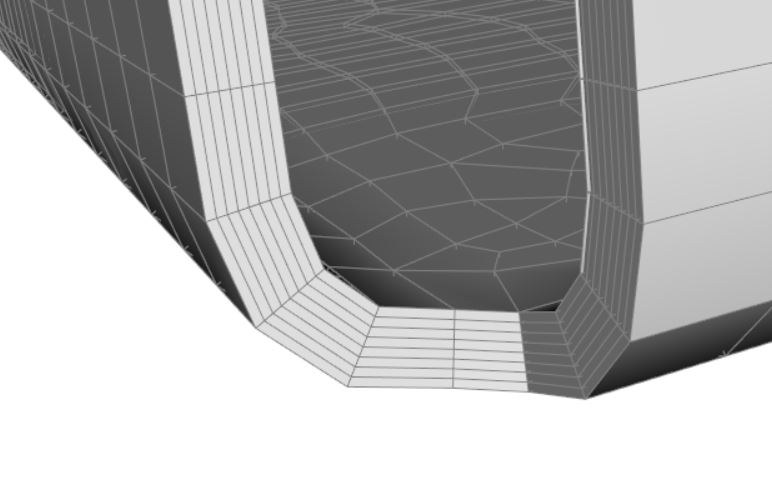
Fig. 4.2 In curved composite parts, it is recommended to use about 5 elements through the thickness in order to get accurate results.
4.4. Material Considerations
The material data of the Mechanical library are typical values and can be used for an initial validation. Because the properties of resin systems very much depend on the manufacturing process, quality and other parameters, it is recommended to run tests to determine empirical values. The different thermal expansion coefficients generate distortions. Thus, it is important to understand that in a curved composite, the expansion coefficients in fiber direction are different than orthogonal to them. In this way, observe the orthotropic thermal properties of the composite material.
4.5. Tool-Part Interaction
Thin and balanced laminates fabricated on flat tooling are often seen to exhibit a concave down curvature.
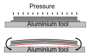
Fig. 4.3 Sketch of a thin laminate that exhibits a concave curvature in the tool side, due to different thermal expansion coefficients.
This is believed to be due to interaction between the laminate and the tool arising because of mismatch between the tool and part coefficient of thermal expansion.
Tool-part interaction in curved laminates can significantly affect spring-in as well as arm bending.
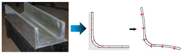
Fig. 4.4 Example of a composite C-Profile and the spring-in effect.
Spring-in increases for laminates cured on male tooling and decreases for laminates cured on female tools
Wrinkling arises on the inner radius when bending the prepreg to conform to the shape of the tool. This can generate substantial stress gradients and distortions when such stresses are locked in the laminate at vitrification
In this way, the tool and the part should be modelled.
It is recommended to have more dynamic cure cycles that require highly responsive tooling, that consider different heating methods (air, liquid, or electric heated tools).
Enhancing the heating area of a heat element can provide more uniform temperature distribution, for example.
4.6. Typical Values and Measurements
The typical value for the thermal film coefficient of air in an autoclave is 5 W/m2 K.
The typical values of the material properties can be found in the typical materials that come with the installation of ACCS. For a correct simulation, it is highly recommended to do the proper measurements of the necessary material properties for each resin.