7. Theory Documentation

During curing of thermosetting composites, the resin undergoes cross-linking reactions that lead to an increase of material density and reduction in volume. A schematic representation of the curing of a thermoset is shown in Figure 1. It traces cure from chain formation and linear growth, through branching and finally to a cross-linked, infinite network. When monomers link into larger molecules they release energy in the form of heat. The exothermic heat of polymerization causes huge problems in processing especially in the case of thick laminates.

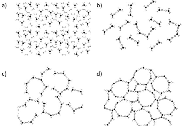
Fig. 7.1 Curing of thermoset resin: a) monomer stage, b) linear growth and branching c) formation of gelled but incompletely cross linked network, d) fully cured thermoset. (From Ref. 1)

7.1. Differential Scanning Calorimetry

Differential Scanning Calorimetry (DSC) is a thermo-analytical technique in which the difference in the amount of heat required to increase the temperature of a sample and reference is measured as a function of temperature. Both the sample and reference are maintained at nearly the same temperature throughout the experiment. Generally, the temperature program for a DSC analysis is designed such that the sample holder temperature increases linearly as a function of time. The reference sample should have a well-defined heat capacity over the range of temperatures to be scanned. The result of a DSC experiment is a curve of heat flux versus temperature or versus time. There are two different conventions: exothermic reactions in the sample shown with a positive or negative peak, depending on the kind of technology used in the experiment. This curve can be used to calculate enthalpies of transitions. This is done by integrating the peak corresponding to a given transition. The heat flow is measured as a direct function of time or of the sample temperature. This data provides extremely valuable information on key physical and chemical properties associated with thermosetting materials, including:

• Glass transition temperature (\(T_{g}\))

• Onset and completion of cure (\(x^{0}\) and \(x^{\infty}\) )

• Total heat of cure (\(H_{R}\))

• Heat capacities (\(C_{p}\))

Different cure kinetics models are available in ACCS. Data obtained through DSC can be fitted to these models. LMAT ltd offers material characterization as a service.

7.2. Cure Kinetics Equations for thermosets

7.2.1. Nth Order

\[\frac{\partial x}{\partial t} = \left(A e^{\frac{-E} {R T}}\right) \left(1-x\right)^n\]

Table 7.1 Parametres’ list

\(x\): Degree of cure \((\%)\)	\(T\): Temperature \((K)\)
\(R\): Universal gas constant \((8.3144621 J.mol^{-1}.K^{-1})\)
\(A\): Pre-exponential factor \((s^{-1})\)	\(E\): Activation energy \((J.mol^{-1})\)
\(n\): Power n \((-)\)

7.2.2. Autocatalytic

\[\frac{\partial x}{\partial t} = \left(A e^{\frac{-E} {R T}}x^m\right) \left(1-x\right)^n\]

Table 7.2 Parametres’ list

\(x\): Degree of cure \((\%)\)	\(T\): Temperature \((K)\)
\(R\): Universal gas constant \((8.3144621 J.mol^{-1}.K^{-1})\)
\(A\): Pre-exponential factor \((s^{-1})\)	\(E\): Activation energy \((J.mol^{-1})\)
\(m\): Power m \((-)\)	\(n\): Power n \((-)\)

7.2.3. Kamal Sourour

\[\frac{\partial x}{\partial t} = \left(A_1 e^{\frac{-E_1} {R T}}+A_2 e^{\frac{-E_2} {R T}} x^m\right) \left(1-x\right)^n\]

Table 7.3 Parametres’ list

\(x\): Degree of cure \((\%)\)	\(T\): Temperature \((K)\)
\(R\): Universal gas constant \((8.3144621 J.mol^{-1}.K^{-1})\)
\(A_{1}, A_{2}\): Pre-exponential factor \((s^{-1})\)	\(E_{1}, E_{2}\): Activation energy \((J.mol^{-1})\)
\(m\): Power m \((-)\)	\(n\): Power n \((-)\)

7.2.4. Avrami-Erofeev

\[\frac{\partial x}{\partial t} = \left(A e^{\frac{-E} {R T}}\right) m \left(1-x\right) \left(-log\left(1-x\right)\right)^{1-1/n}\]

Table 7.4 Parametres’ list

\(x\): Degree of cure \((\%)\)	\(T\): Temperature \((K)\)
\(R\): Universal gas constant \((8.3144621 J.mol^{-1}.K^{-1})\)
\(A\): Pre-exponential factor \((s^{-1})\)	\(E\): Activation energy \((J.mol^{-1})\)
\(m\): Power m \((-)\)	\(n\): Power n \((-)\)

7.2.5. Karnakas-Partridge

\[\frac{\partial x}{\partial t} = A_1 e^{\frac{-E_1} {R T}}\left(1-x\right)^{n^1}+A_2 e^{\frac{-E_2} {R T}} x^m\left(1-x\right)^{n^2}\]

Table 7.5 Parametres’ list

\(x\): Degree of cure \((\%)\)	\(T\): Temperature \((K)\)
\(R\): Universal gas constant \((8.3144621 J.mol^{-1}.K^{-1})\)
\(A_{1}, A_{2}\): Pre-exponential factor \((s^{-1})\)	\(E_{1}, E_{2}\): Activation energy \((J.mol^{-1})\)
\(m\): Power m \((-)\)	\(n_{1}, n_{2}\): Power n \((-)\)

7.2.6. Proportional Diffusion Limitation

\[difLim = 1+e^{C\left(x-\left(AC_0+AC_{T} T\right)\right)}\]

Table 7.6 Parametres’ list

\(x\): Degree of cure \((\%)\)	\(T\): Temperature \((K)\)
\(AC_{0}\): Initial value \((-)\)	\(AC_{0}\): Temperature dependence \((K^{-1})\)
\(C\): Coefficient C \((-)\)

7.2.7. Parallel Diffusion Limitation

\[difLim = A_{D} e^{-\frac{E_D} {R T} e^{-\frac{-b} {w \left(T-T_{g}\right)+g}}}\]

Table 7.7 Parametres’ list

\(T\): Temperature \((K)\)	\(T_{g}\): Glass transition temperature \((K)\)
\(R\): Universal gas constant \((8.3144621 J.mol^{-1}.K^{-1})\)
\(A_{D}\): Pre-exponential factor \((s^{-1})\)	\(E_{D}\): Activation energy \((J.mol^{-1})\)
\(b\): Coefficient b \((-)\)	\(w\): Coefficient w \((K^{-1})\)
\(g\): Coefficient g \((-)\)

7.2.8. Released Heat

\[\dot{q} = \frac{H_R\rho\left(1-V_f\right)}{x^\infty} \frac{\partial x}{\partial t}\]

Table 7.8 Parametres’ list

\(H_R\): Total heat of reaction \((J kg^{-1})\)	\(\rho\): Mass density \((kg.m^{-3})\)
\(V_{f}\): Fibre volume fraction \((-)\)	\(x^{\infty}\): Maximum degree of cure \((\%)\)

7.2.9. Glass Transition Temperature

\[T_{g} = T^{0}_{g}+\lambda x \frac {T^{\infty}_{g}-T^{0}_{g}} {1-\left(1-\lambda\right)x}\]

Table 7.9 Parametres’ list

\(T^{0}_{g}\): Initial value \((K)\)	\(T^{\infty}_{g}\): Final value \((K)\)
\(\lambda\): Fitting coefficient \((-)\)	\(x\): Degree of cure \((\%)\)

7.2.10. Cure Shrinkage

\[\Delta{}\varepsilon_{X} = \Delta{}x \varepsilon^{sh}_X\]

\[\Delta{}\varepsilon_{Y} = \Delta{}x \varepsilon^{sh}_Y\]

\[\Delta{}\varepsilon_{Z} = \Delta{}x \varepsilon^{sh}_Z\]

Table 7.10 Parametres’ list

\(x\): Degree of cure \((\%)\)	\(\varepsilon^{sh}_{x}\): Total cure shrinkage normal strain alon X \((-)\)
\(\varepsilon^{sh}_{y}\): Total cure shrinkage normal strain alon Y \((-)\)	\(\varepsilon^{sh}_{z}\): Total cure shrinkage normal strain alon Z \((-)\)

The user can only provide directional cure shrinkage strains. The cure shrinkage is scaled linearly with the degree of cure \(x\).

7.2.11. Material Model

There are generally two main transitions that can be identified during the curing process of a thermosetting resin. The first one is gelation occurring at approximately 30% - 50% degree of conversion and the second one is vitrification occurring when the current temperature becomes lower than the glass transition temperature (\(T_{g}\)). Gelation is an irreversible process and corresponds to the formation of a 3-D infinite network of polymer chains. Vitrification occurs once the current temperature becomes lower than the glass transition temperature (\(T_{g}\)) and the resin transforms from the rubbery to the glassy, or solid, state. Vitrification is reversible and when the material temperature exceeds \(T_{g}\), the epoxy transforms back from the glassy to the rubbery state.

The thermoset material model within ACCS has four material states: liquid, un-gelled glassy, rubbery, and glassy as illustrated in Figure 1. Liquid has a state value of 0, un-gelled glassy of 1, rubbery of 2 and glassy of 3. The continuous blue line corresponds to the glass temperature transition, the green line to the gelation degree of cure, and the red numbers highlight the zone where the sub-equations are valid. A smooth variation of material properties can be used by setting strictly positive values to the margins \(T_{m}\) and \(x_{m}\). It will linearly interpolate between the properties of the different material states according to the temperature, glass transition temperature, degree of cure, and gelation degree of cure in thermosets.

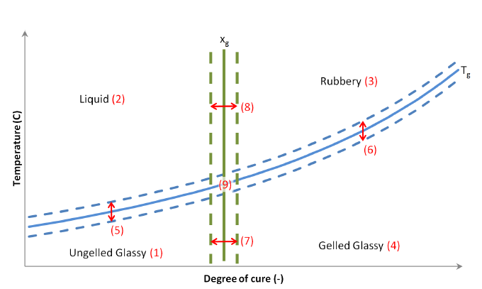
Fig. 7.2 Temperature vs. Degree of cure plot highlighting the material states

The variables used to compute the material properties are:

Table 7.11 Properties’ list

\(T\): Temperature \((K)\)	\(x\): Degree of cure \((-)\)
\(T_{g}\): Glass transition temperature \((K)\)	\(x_{g}\): Gelation degree of cure \((-)\)
\(T_{m}\): Margin around glass transition temperature \((\Delta K)\)	\(x_{m}\): Margin around gelation degree of cure \((-)\)

A material property named “A” have the following names in the different states:

Table 7.12 Property denomination for each material state

\(A^{L}\): Property in liquid state	\(A^{U}\): Property in ungeled glassy state
\(A^{R}\): Property in rubbbery state	\(A^{S}\): Property in geled glassy state

\[\begin{split}A = \begin{cases} A^{U} & \text{if} & x \leq x_{g}-x_{m} & \text{and} & T \leq T_{g}-T_{m} & (1)\\ A^{L} & \text{if} & x \leq x_{g}-x_{m} & \text{and} & T_{g}+T_{m} \leq T & (2)\\ A^{R} & \text{if} & x_{g}+x_{m} \leq x & \text{and} & T \leq T_{g}-T_{m} & (3)\\ A^{S} & \text{if} & x_{g}+x_{m} \leq x & \text{and} & T_{g}+T_{m} \leq T & (4)\\ \frac{1}{2}\left[ A^{U}\frac{T-T_{m}}{T_{g}-T_{m}} + A^{L}\frac{T+T_{m}}{T_{g}-T_{m}} \right] & \text{if} & x \leq x_{g}-x_{m} & \text{and} & T_{g}-T_{m} < T < T_{g}+T_{m} & (5)\\ \frac{1}{2}\left[ A^{S}\frac{T-T_{m}}{T_{g}-T_{m}} + A^{R}\frac{T+T_{m}}{T_{g}-T_{m}} \right] & \text{if} & x_{g}+x_{m} \leq x & \text{and} & T_{g}-T_{m} < T < T_{g}+T_{m} & (6)\\ \frac{1}{2}\left[ A^{U}\frac{x-x_{m}}{x_{g}-x_{m}} + A^{S}\frac{x+x_{m}}{x_{g}-x_{m}} \right] & \text{if} & x_{g}-x_{m} < x < x_{g}+x_{m} & \text{and} & T \leq T_{g}-T_{m} & (7)\\ \frac{1}{2}\left[ A^{L}\frac{x-x_{m}}{x_{g}-x_{m}} + A^{R}\frac{x+x_{m}}{x_{g}-x_{m}} \right] & \text{if} & x_{g}-x_{m} < x < x_{g}+x_{m} & \text{and} & T_{g}+T_{m} \leq T & (8)\\ \frac{1}{4}\left[ A^{L}\frac{x-x_{m}}{x_{g}-x_{m}}\frac{T+T_{m}}{T_{g}-T_{m}} + A^{U}\frac{x-x_{m}}{x_{g}-x_{m}}\frac{T-T_{m}}{T_{g}-T_{m}} + A^{R}\frac{x+x_{m}}{x_{g}-x_{m}}\frac{T+T_{m}}{T_{g}-T_{m}} + A^{S}\frac{x+x_{m}}{x_{g}-x_{m}}\frac{T-T_{m}}{T_{g}-T_{m}} \right] & \text{if} & x_{g}-x_{m} < x < x_{g}+x_{m} & \text{and} & T_{g}-T_{m} < T < T_{g}+T_{m} & (9)\\ \end{cases}\end{split}\]

7.3. Crystallisation Equations for thermoplastics

7.3.1. PEEK

The implementation of the PEEK material model is based on the work published by Velisaris and Seferis [PEEK_ref].

\[x^{t} = x^{\infty} \left( w^{N} F^{N}_{vc} + \left(1-w^{N}\right) F^{G}_{vc} \right)\]

\[x^{t} = x^{c} \left( 1 - \frac{K_{int}}{2} \right)\]

\[F^{X}_{vc} = 1-e^{-\left( \left(log\left({\frac{1}{1-F^{X}_{vc}}}\right)\right)^{\frac{1}{n^{X}}} + \delta t \left(K^{X}\right)^{\frac{1}{n^{X}}} \right)^{n^{X}}}\]

\[K_{int} += \left( A_{m} e^{-\frac{E_{m}} {R T}} \right) \delta t\]

\[K^{X} = C^{X}_{1} T e^{-\frac{C^{X}_{2}}{T-\left(T_{g}+dT_{g}\right)} - \frac{C^{X}_{3}}{T\left(T_{g}-T^{X}_{m}\right)}}\]

\[F^{X}_{vc} = F^{X}_{vc} \frac{x^{t}} {x^{t-\delta t}}\]

Table 7.13 Parametres’ list

\(x^{t}\): Degree of crystallisation \((\%)\)	\(x^{\infty}\): Maximum degree of crystallisation \((\%)\)
\(x^{c}\): Degree of crystallisation at end of crystallisation \((\%)\)	\(K_{int}\): Integral of Arrhenius law \((s)\)
\(w^{N}\): Nucleation weight factor \((-)\)	\(X\): Nucleation (N) or Growth (G) upper index \((-)\)
\(F^{X}_{vc}\): Growth normalized volume fraction of crystallinities \((-)\)	\(n^{X}\): Avrami exponent \((-)\)
\(K^{X}\): Crystallisation rate \((s^{-n^{X}})\)	\(C_{1}^{X}\): Constant C1 \((s^{-n^{X}}.K^{-1})\)
\(C_{2}^{X}\): Constant C2 \((K)\)	\(C_{3}^{X}\): Constant C3 \((K^{3})\)
\(T_{m}^{X}\): Melting temperature \((K)\)
\(T\): Temperature \((K)\)	\(\delta t\): Time step \((s)\)
\(T_{g}\): Glass transition temperature \((K)\)	\(dT_{g}\): Glass transition temperature shift \((\Delta K)\)
\(A_{m}\): Pre-exponential factor \((s^{-1})\)	\(E_{m}\): Activation energy \((J.mol^{-1})\)

7.3.2. Released Heat

\[\dot{q} = \frac{H_R\rho\left(1-V_f\right)}{x^\infty} \frac{\partial x}{\partial t}\]

Table 7.14 Parametres’ list

\(H_R\): Total heat of reaction \((J kg^{-1})\)	\(\rho\): Mass density \((kg.m^{-3})\)
\(V_{f}\): Fibre volume fraction \((-)\)	\(x^{\infty}\): Maximum degree of crystallisation \((\%)\)

7.3.3. Reference Temperature

\[T_{r} = T^{am}_{r}+ \left(T^{cr}_{r}-T^{am}_{r}\right) \frac {x} {x^{\infty}}\]

Table 7.15 Parametres’ list

\(T^{am}_{r}\): Amorphous reference temperature \((K)\)	\(T^{cr}_{r}\): Crystallised reference temperature \((K)\)
\(x\): Degree of crystallisation \((\%)\)	\(x^{\infty}\): Maximum degree of crystallisation \((\%)\)

7.3.4. Cure Shrinkage

The volume variation is computed by the following equation:

\[\Delta V = \frac{\Delta \rho}{\rho}\]

Table 7.16 Parametres’ list

\(\Delta \rho\): Mass density variation \((K)\)

\(\rho\): Mass density \((kg.m^{-3})\)

The linear cure shrinkage of the matrix is computed by the following equation:

\[\Delta\varepsilon^{sh}_{m} = \frac { -1 + \sqrt{1+\frac{4}{3}\Delta V}} {2}\]

The linear cure shrinkage of the mix is computed by the following equations:

\[\Delta\varepsilon_{X} = \frac { E_{m} \Delta\varepsilon^{sh}_{m} \left(1-V_{f}\right) } { E^{XX}_{f}V_{f}+E_{m}\left(1-V_{f}\right) }\]

\[\Delta\varepsilon_{Y} = \Delta\varepsilon_{Z} = \left(1+\nu_{m}\right)\Delta\varepsilon^{sh}_{m}\left(1-V_{f}\right) - \Delta\varepsilon_{X} \left(\nu^{XY}_{f}V_{f}+\nu_{m}\left(1-V_{f}\right)\right)\]

Table 7.17 Parametres’ list

\(E_{m}\): Young’s modulus of the matrix \((Pa)\)	\(\nu_{m}\): Poisson’s ratio of the matrix \((-)\)
\(E^{XX}_{f}\): Young’s modulus of the fibres \((Pa)\)	\(\nu^{XY}_{f}\): Poisson’s ratio of the fibres \((-)\)
\(V_{f}\): Fibre volume fraction \((-)\)

7.3.5. Material Model

In thermoplastics there are generally two main transitions that can be identified during the curing process. The first one is crystallisation occurring when the current temperature becomes lower than the glass transition temperature (\(T_{g}\)) and the second one is melting occurring when the current temperature becomes higher than the melting temperature (\(T_{m}\)). The crystallisation occurs once the current temperature becomes lower than the glass transition temperature (\(T_{g}\)) and the resin transforms from the crystallisation to the glassy, or solid, state. The crystallisation is reversible and when the material temperature exceeds \(T_{g}\), the resin transforms back from the glassy to the crystallisation state. Melting occurs once the current temperature becomes higher than the melting temperature (\(T_{m}\)) and the polymer transforms from the crystallisation to the melted, state. Melting is irreversible and the crystallisation is reset to 0 when the material is in the melting state.

The material model within ACCS has four material states: glassy, lower crystallisation, higher crystallisation, and melted as illustrated in Figure 1. Glassy has a state value of -1, lower crystallisation glassy of 0, higher crystallisation of 1 and melted of 2.

7.4. Viscoelasticity

ACCS can take into account viscoelasticity during curing. They are defined for each material state (\(s\)) and on the stiffnesses of the three normal and the three shearing directions (\(ij\)). The instantaneous modulus (\(A^{0}_{ij}\)) is obtained by the mixing rule described in Material Model.

Note: Viscoelasticity is only supported for thermosets currently.

7.4.1. Maxwell Model

Effective stiffnesses:

\[A^{s}_{ij}=A^{0}_{ij}\]

Table 7.18 Parametres’ list

\(A^{0}_{ij}\): Instantaneous modulus \((Pa)\)

Viscoelastic increment:

\[\delta \varepsilon v^{s}_{ij} = \left(1-e^{-\delta t/\tau^{s}_{ij}}\right)\left(\varepsilon_{ij}-\varepsilon v^{s}_{ij}\right)\]

Table 7.19 Parametres’ list

\(\delta t\): Time step \((s)\)	\(\tau^{s}_{ij}\): Time constant \((s)\)
\(\varepsilon_{ij}\): Mechanical strain value at beginning of time step \((-)\)	\(\varepsilon v^{s}_{ij}\): Viscoelastic strain value at beginning of time step \((-)\)

7.4.2. Power Law

Effective stiffnesses:

\[A^{s}_{ij}=A^{0}_{ij} C^{s}_{ij}\]

Table 7.20 Parametres’ list

\(A^{0}_{ij}\): Instantaneous modulus \((Pa)\)

\(C^{s}_{ij}\): Modulus coefficient \((-)\)

Viscoelastic increment:

\[\delta \varepsilon v^{s}_{ij} = \left(\delta t\right)^{-n^{s}_{ij}}\]

Table 7.21 Parametres’ list

\(\delta t\): Time step \((s)\)

\(n^{s}_{ij}\): Power n \((-)\)

7.4.3. Prony Series

Effective stiffness’s for each terms (u):

\[A^{us}_{ij}=A^{0}_{ij}C^{us}_{ij}\]

Table 7.22 Parametres’ list

\(A^{0}_{ij}\): Instantaneous modulus \((Pa)\)

\(C^{us}_{ij}\): Modulus coefficient \((-)\)

Visco-elastic strain increment:

\[\delta \varepsilon v^{us}_{ij} = \left(1-e^{-\frac{\delta t}{\tau^{us}_{ij}}}\right)\left(\varepsilon_{ij}-\varepsilon v^{us}_{ij}\right)\]

Table 7.23 Parametres’ list

\(\delta t\): Time step \((s)\)	\(\tau^{us}_{ij}\): Time constant \((s)\)
\(\varepsilon_{ij}\): Mechanical strain value at beginning of time step \((-)\)	\(\varepsilon v^{us}_{ij}\): Viscoelastic strain value at beginning of time step \((-)\)

7.4.4. Extended Standard Non-Linear Series

Effective stiffness’s for each terms (u):

\[A^{us}_{ij}=A^{0}_{ij} C^{us}_{ij}\]

Table 7.24 Parametres’ list

\(A^{0}_{ij}\): Instantaneous modulus \((Pa)\)

\(C^{us}_{ij}\): Modulus coefficient \((-)\)

Visco-elastic strain increment:

\[\delta \varepsilon v^{us}_{ij} = \left(1-\left(e^{-\frac{\delta t}{\tau^{us}_{ij}}}\right)^{n^{us}_{ij}}\right) \left(\varepsilon_{ij}-\varepsilon v^{us}_{ij}\right)\]

Table 7.25 Parametres’ list

\(\delta t\): Time step \((s)\)
\(\tau^{us}_{ij}\): Time constant \((s)\)	\(n^{s}_{ij}\): Power n \((-)\)
\(\varepsilon_{ij}\): Mechanical strain value at beginning of time step \((-)\)	\(\varepsilon v^{us}_{ij}\): Viscoelastic strain value at beginning of time step \((-)\)

7.4.5. Temperature Time Shift

\[\begin{split}t = \begin{cases} t / 10 ^{ A_{1} \left(T-T_{MID}\right) + C_{1} \frac{T_{MID}-T_{R}}{C_{2}+T_{MID}-T_{R}} }, & \text{if}\ T < T_{MID} \\ t / 10 ^{ C_{1} \frac{T-T_{R}}{C_{2}+T-T_{R}} }, & \text{if}\ T \geq T_{MID} \end{cases}\end{split}\]

Table 7.26 Parametres’ list

\(T\): Temperature \((K)\)	\(T_{MID}\): Mid-point temperature \((K)\)
\(T_{R}\): Reference temperature \((K)\)	\(A_{1}\): Coefficient \((-)\)
\(C_{1}\): Coefficient \((-)\)	\(C_{2}\): Coefficient \((K)\)

7.4.6. Degree of Cure Time Shift

\[t = t / 10^{ D_{1}\left(1-e^{D_{2}\left(1-x\right)}\right) }\]

Table 7.27 Parametres’ list

\(x\): Degree of cure \((\%)\)
\(D_{1}\): Coefficient D1 \((-)\)	\(D_{2}\): Coefficient D2 \((-)\)

7.5. References

PEEK_ref

Velisaris, C.N. and Seferis, J.C. (1986), crystallisation kinetics of polyetheretherketone (peek) matrices. Polym Eng Sci, 26: 1574-1581. doi:10.1002/pen.760262208