You can view this "What's New" page in your system browser instead of the Mechanical environment using the link below. Additionally, the browser version will include any content updated since the release of Mechanical 2021 R1.

Browser version of this "What's New" page

"What's New" for Previous Mechanical Releases

Use these links to easily see the "What's New" pages for previous releases of Mechanical. Use the first link to return to this "2021 R1 What's New" page.

2021 R1 What's New (You are here)

Helpful Links

These are for your convenience. They require internet access and will open in a new browser window. Some also require Ansys Customer Portal login credentials.

Mechanical Technology Showcase

A New Collection of Example Problems Showcasing Mechanical's Technology

The Technology Showcase: Example Problems guidebook is a new collection of real-world problems from a wide range of industries and engineering disciplines. Learn various features and recommendations for using ANSYS Mechanical to solve complex problems. Explore the solutions hands-on with the downloadable input and workbench project archive files in this new demonstration guidebook.

mortarboard cap Want to learn more? If you are on Windows, go to the documentation for this topic.
(Requires internet access and will open in a new browser window. Not for Linux platforms.)

Geometry

Modeling Slender Cable Structures

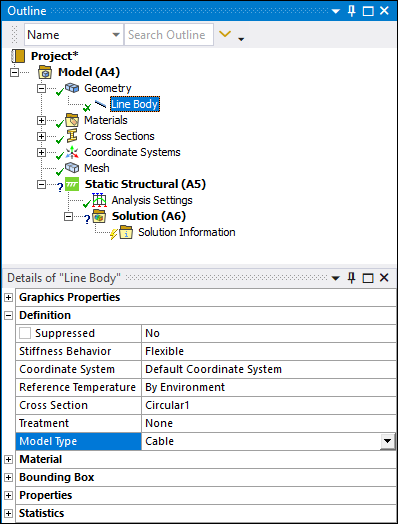
Cable-type line bodies now use higher-order elements by default. Specifically, the program-controlled element order setting for cables is the quadratic CABLE280 element rather than the linear LINK180 element. Quadratic elements produce higher rates of convergence and increase results accuracy. The application will continue using the LINK180 element when the global element order is linear.

mortarboard cap Want to learn more? If you are on Windows, go to the documentation for this topic.
(Requires internet access and will open in a new browser window. Not for Linux platforms.)

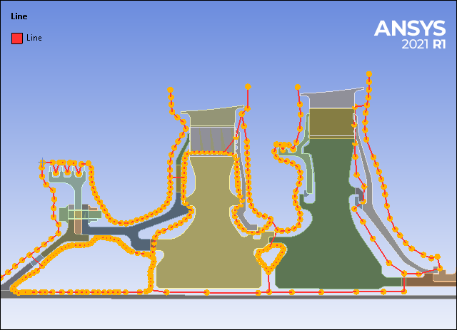
Creating Line Bodies

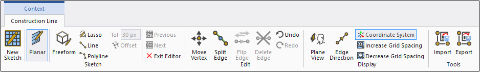
The Construction Geometry feature now has an option, Line, that enables you to create line bodies. This new option creates an object with sketching tools for creating line-segments that you can convert into line bodies.

This feature is useful when you want to quickly add line bodies to your model, such as when you want to define a fluid network to model flow and heat transfer.

A valuable accompanying feature to creating lines bodies is the ability to import and overlay a reference image on your model. This enables you to accurately sketch (trace) line bodies on and around your model.

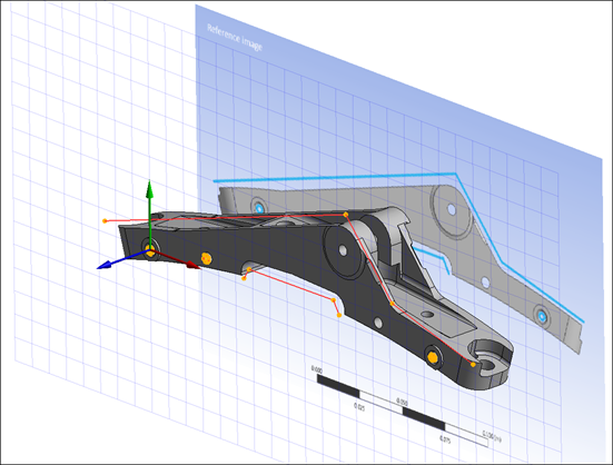
In addition, this feature supports API for scripting and can be recorded (using the new recording feature).

mortarboard cap Want to learn more? If you are on Windows, go to the documentation for this topic.
(Requires internet access and will open in a new browser window. Not for Linux platforms.)

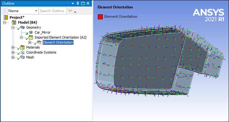
Importing Element Orientations

You can now import coordinate system data points from an External Data system onto the elements of your model in the form of Element Orientations so that you can control how the material properties vary across the model. This feature also provides access to a new mapping option: Quaternion. This option interpolates the orientations in the quaternion space rather than directly on the Euler angles.

mortarboard cap Want to learn more? If you are on Windows, go to the documentation for this topic.
(Requires internet access and will open in a new browser window. Not for Linux platforms.)

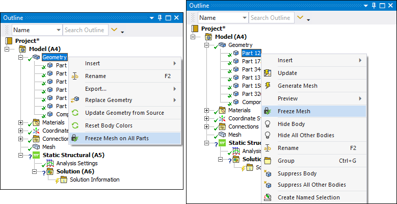
Freezing the Mesh on Parts

There are new Geometry and Part object options available to freeze (and unfreeze) the mesh of all geometry parts or selected parts of your model. The feature restricts any changes to the mesh of specified parts while active.

mortarboard cap Want to learn more? If you are on Windows, go to the documentation for this topic.
(Requires internet access and will open in a new browser window. Not for Linux platforms.)

Materials

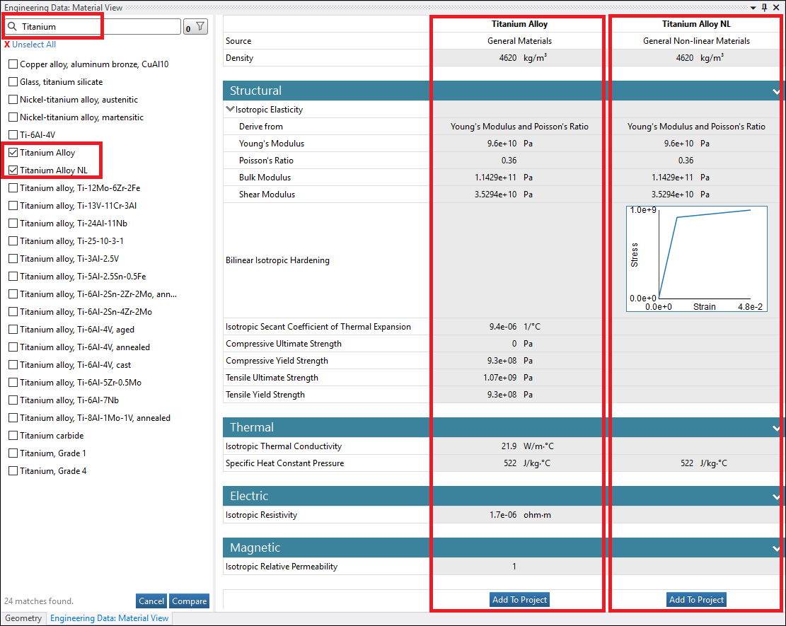
Comparing Engineering Data Materials

You can now compare materials in Engineering Data! Use search and filter tools to show side-by-side properties of selected materials for easy comparison.

mortarboard cap Want to learn more? If you are on Windows, go to the documentation for this topic.
(Requires internet access and will open in a new browser window. Not for Linux platforms.)

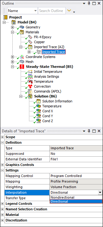
Imported Trace

The Imported Trace object has a new interpolation capability. Using the new Directional option of the Interpolation property, you can calculate the effective orthotropic conductivity for each element using the position and values of the trace data within each element. The behavior from a previous release is still available using the Nondirectional option that calculates effective conductivity by averaging the trace data in each element.

mortarboard cap Want to learn more? If you are on Windows, go to the documentation for this topic.
(Requires internet access and will open in a new browser window. Not for Linux platforms.)

Contact and Connections

Contact Region Scoping

You can now scope the Contact side of a Contact Region to mesh nodes. This scoping capability supports the Geometry and Named Selection scoping methods.

mortarboard cap Want to learn more? If you are on Windows, go to the documentation for this topic.
(Requires internet access and will open in a new browser window. Not for Linux platforms.)

Edge-to-Edge and Edge-to-Surface Contact

Now, for edge-to-edge and edge-to-surface contact during a 3D analysis, the application supports the line contact element CONTA177. You use the new property, Edge Contact Type, to specify the desired element type for the Contact geometry.

mortarboard cap Want to learn more? If you are on Windows, go to the documentation for this topic.
(Requires internet access and will open in a new browser window. Not for Linux platforms.)

Interface Treatment

The options listed below are now available for the Interface Treatment property of the Geometric Modification category of the Contact Region object. These options enable you to apply Offset values, once the application closes any gaps or penetrations at the contact interface, with or without regard to initial contact status (near open/open/closed).

Offset Only, Ramped Effects
Offset Only, No Ramping
Offset Only, Ignore Initial Status, Ramped Effects
Offset Only, Ignore Initial Status, No Ramping

mortarboard cap Want to learn more? If you are on Windows, go to the documentation for this topic.
(Requires internet access and will open in a new browser window. Not for Linux platforms.)

Remote Point

You can now scope a Remote Point object to Element Faces.

mortarboard cap Want to learn more? If you are on Windows, go to the documentation for this topic.
(Requires internet access and will open in a new browser window. Not for Linux platforms.)

External Model

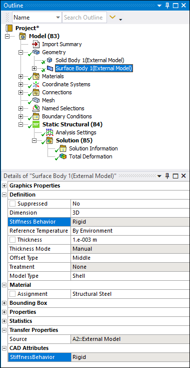
Importing Rigid Bodies from ABAQUS

The External Model system now enables you to import rigid body definitions from ABAQUS files (*RIGID BODY command).

mortarboard cap Want to learn more? If you are on Windows, go to the documentation for this topic.
(Requires internet access and will open in a new browser window. Not for Linux platforms.)

New Spring Connection Element

The application now enables you to import the nonlinear spring element, COMBIN39, from ANSYS CBD files. Certain restrictions apply.

mortarboard cap Want to learn more? If you are on Windows, go to the documentation for this topic.
(Requires internet access and will open in a new browser window. Not for Linux platforms.)

Mesh

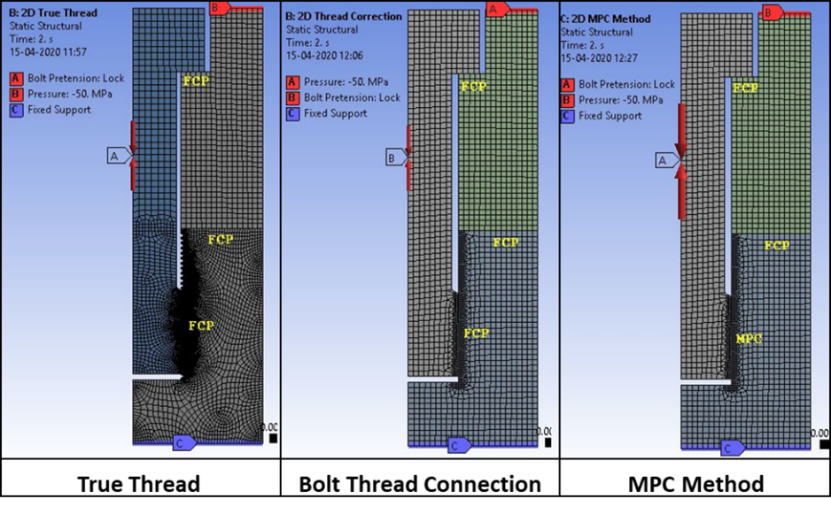
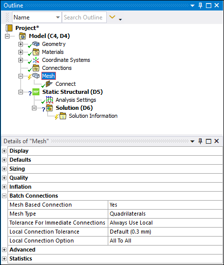
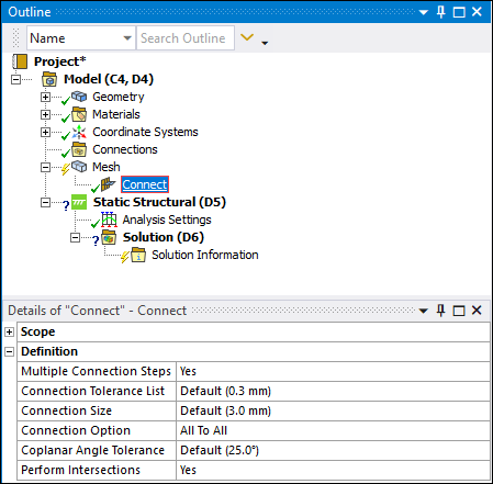
Mesh Based Connections

For beam and shell assemblies, the Multiple Connection Steps, Connection Tolerance List, Connection Size, and Coplanar Angle Tolerance properties have been moved from the Mesh object to the new Connect object. This new object provides the functionalities (therefore creating a conformal mesh between the selected entities) that were previously available at the global level when the Mesh Based Connections property was set to On.

mortarboard cap Want to learn more? If you are on Windows, go to the documentation for this topic.
(Requires internet access and will open in a new browser window. Not for Linux platforms.)

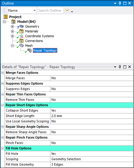
Repair Topology

The Repair Topology feature enables you to defeature your model at the mesh level when the Mesh Based Connections property is set to Yes. The object has two new Details categories: Repair Short Edges Options and Fill Hole Options. The Repair Short Edges Options enable you to collapse edges below the specified Short Edge Length and the Fill Hole Options enables you to remove holes using scoped edge loops.

mortarboard cap Want to learn more? If you are on Windows, go to the documentation for this topic.
(Requires internet access and will open in a new browser window. Not for Linux platforms.)

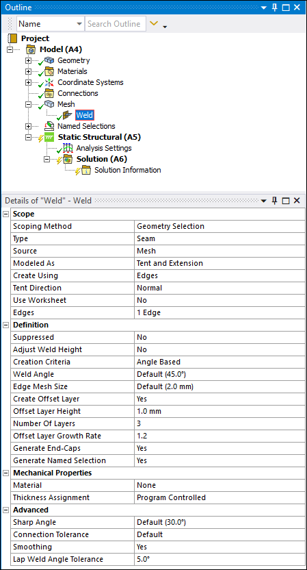
Weld

The Weld object has several new capabilities. The direction in which a tent face gets created can now be controlled by the Tent Direction property. The Number of Layers property now allows up to three layers for all Modeled As property options. The Weld object can automatically assign thicknesses to generated weld bodies based on the parent bodies connected by them. And you can now import and export .csv files from the Worksheet enabling you to work with many welds.

mortarboard cap Want to learn more? If you are on Windows, go to the documentation for this topic.
(Requires internet access and will open in a new browser window. Not for Linux platforms.)

Analysis

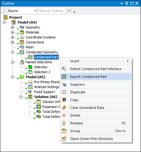
Exporting Condensed Parts

The application now supports the “bottom-up” substructuring approach by enabling you to export generated superelements using the new Export Condensed Part option. Your exported superelements can then be imported into a different Mechanical session.

mortarboard cap Want to learn more? If you are on Windows, go to the documentation for this topic.
(Requires internet access and will open in a new browser window. Not for Linux platforms.)

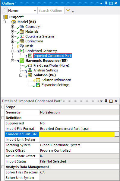
Importing Condensed Parts

To support bottom-up substructuring, the new Imported Condensed Part object can be added through the Condensed Geometry object. For your current session, this enables you to import superelements and connect them to the rest of your model. You can then perform the use pass on this assembled model.

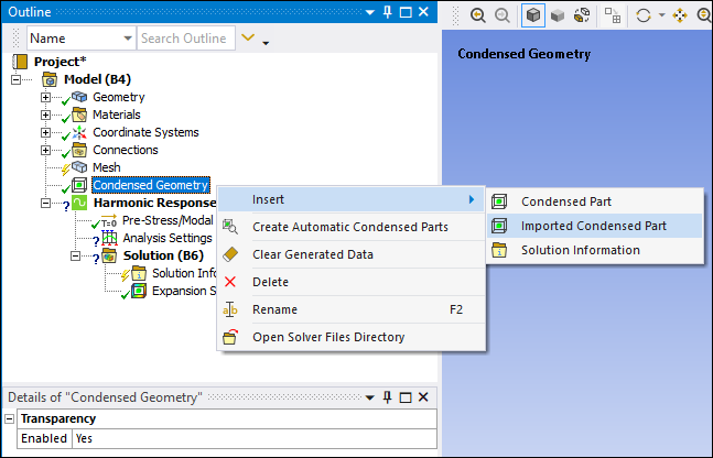
Once inserted, specify the desired Condensed Part file to import.

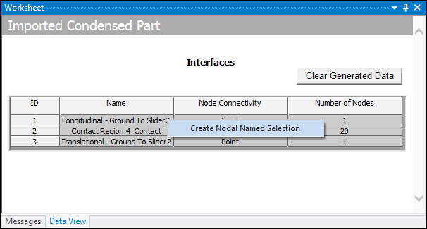
Once imported, the Worksheet provides a right-click option to create Element and Nodal Named Selections for each interface. These named selections can then be used to define connections and/or boundary conditions.

mortarboard cap Want to learn more? If you are on Windows, go to the documentation for this topic.
(Requires internet access and will open in a new browser window. Not for Linux platforms.)

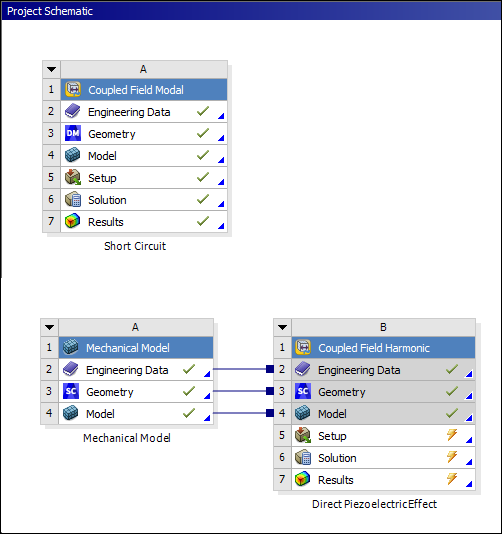
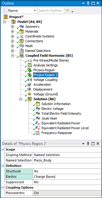
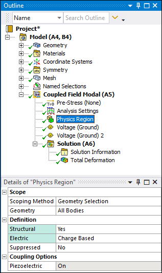
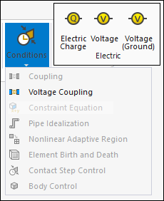
Piezoelectric Analysis

You can now perform piezoelectric coupling between electric and structural physics using the Coupled Field Harmonic and Coupled Field Modal analyses. The Piezoelectric coupling is specified using the Physics Region object and enabling both Structural and Electric physics.

In Engineering Data the new material properties Piezoelectric Matrix, Anisotropic Elasticity, and Relative Permittivity, support these analyses. The Piezoelectric Matrix and Anisotropic Elasticity material properties support data in both IEEE and MAPDL format.

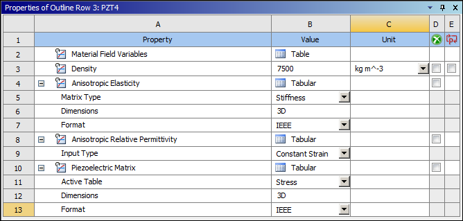
These analysis types now support Electric Capacitance for contact conditions.

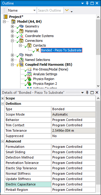
These analysis types also include the new Electric Charge, Voltage, and Voltage (Ground) loading conditions as well as the new Voltage Coupling boundary condition.

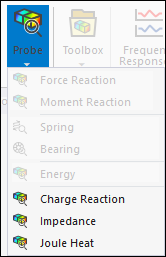
The Coupled Field Harmonic analysis supports Frequency Response and the Probe results for Charge Reaction and Impedance.

mortarboard cap Want to learn more? If you are on Windows, go to the documentation for this topic.
(Requires internet access and will open in a new browser window. Not for Linux platforms.)

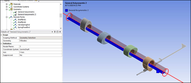
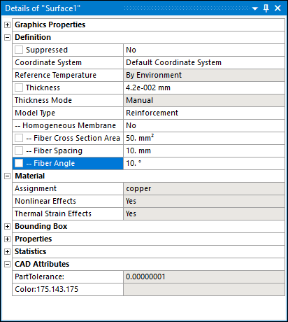
Reinforcement Analysis Enhancements

The capability to specify line bodies and surface bodies within a base structure as reinforcements has been expanded to include the following three-dimensional analysis types:

Modal (Standalone and Pre-Stressed)
Harmonic Analysis (Standalone, Pre-Stressed, and MSUP)
Random Vibration

Furthermore, you can now specify the orientation of fibers for a surface body reinforcement with the new Fiber Angle property (when Homogenous Membrane is set to No).

mortarboard cap Want to learn more? If you are on Windows, go to the documentation for this topic.
(Requires internet access and will open in a new browser window. Not for Linux platforms.)

Loading and Support Conditions

Boundary Condition Finite Element Scoping

You can now scope the following boundary conditions to finite element entities (elements, element faces, or nodes), including finite element-based Named Selections or finite element-based Remote Points:

Bearing (3D element faces only)
Bolt Pretension (elements and element faces)
Displacement (element faces and nodes)
Force (3D element faces only and nodes)
Imported Convection Coefficient (element faces)
Imported Temperature (element faces)
Moment (element faces and nodes)
Pressure (3D element faces only and nodes)
Remote Displacement (element faces and nodes)
Remote Force (element faces and nodes)
Thermal Condition (elements)

mortarboard cap Want to learn more? If you are on Windows, go to the documentation for this topic.
(Requires internet access and will open in a new browser window. Not for Linux platforms.)

Direct Loading when a Cyclic Region is Specified

For a Cyclic Symmetry analysis that includes a Cyclic Region, you can now apply Pressure, Force, and Imported Pressure loads directly on bodies using the Applied By property, without creating surface effect elements.

mortarboard cap Want to learn more? If you are on Windows, go to the documentation for this topic.
(Requires internet access and will open in a new browser window. Not for Linux platforms.)

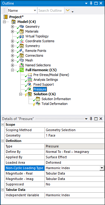
Non-Cyclic Loading Support for Cyclic Symmetry

Now, during a Full Harmonic Response analysis that includes cyclic symmetry (Cyclic Region object present), you can specify non-cyclic loading using the new Non-Cyclic Loading Type property. This new type of loading, also known as engine-order loading (or traveling wave excitation), excites one or more harmonic indices.

mortarboard cap Want to learn more? If you are on Windows, go to the documentation for this topic.
(Requires internet access and will open in a new browser window. Not for Linux platforms.)

Imported CFD Pressure

A new loading condition is now available for Harmonic Acoustic analyses: Imported CFD Pressure. This boundary condition enables you to map and apply the pressure loading data contained in a Fluent-Mechanical coupling data file (.cgns) on your model.

mortarboard cap Want to learn more? If you are on Windows, go to the documentation for this topic.
(Requires internet access and will open in a new browser window. Not for Linux platforms.)

Solution

Solution Information

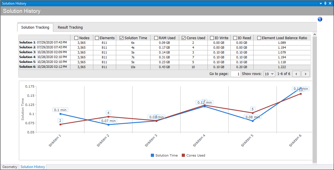
The Solution Information object has a new Solution History option for the Solution Output property.

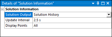
When selected, this option displays a Worksheet that contains two tabs to review solution performance information and results: Solution Tracking and Result Tracking. The Solution Tracking tab tracks solution time, computational resources used, and the number of nodes and elements for each solution.

The Result Tracking tab tracks a result's minimum and maximum values and the number of nodes and elements for each solution.

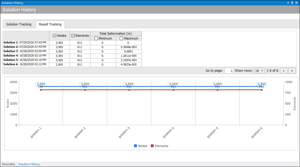
Each tab presents a chart that graphs the data contained in the columns you select in the table. Each table heading provides a filter as well as a check box. Only two check boxes can be selected at one time. You can change chart display settings (lines or columns) as well as the labeling by right-clicking in the chart.

mortarboard cap Want to learn more? If you are on Windows, go to the documentation for this topic.
(Requires internet access and will open in a new browser window. Not for Linux platforms.)

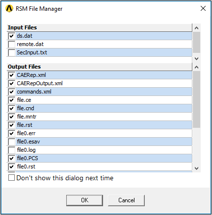
Remote Solution File Download Selection

Now, when you perform a solution remotely, you can choose to display the RSM File Manager dialog. This dialog enables you to select or clear the input/output files you wish to download from the remote location.

mortarboard cap Want to learn more? If you are on Windows, go to the documentation for this topic.
(Requires internet access and will open in a new browser window. Not for Linux platforms.)

Results and Post Processing

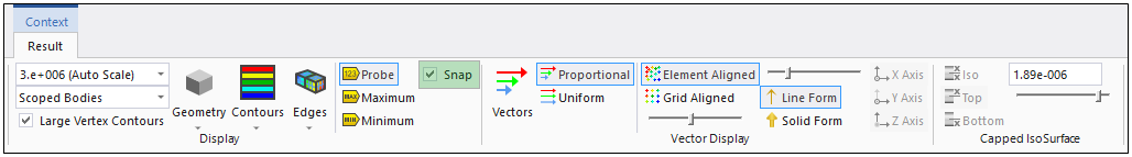
Automatic Probe Annotation Placement

Now, when you are using the Probe option to place annotations on results, there is a new accompanying Snap option. This option automatically places (snaps) the annotation on the nearest mesh node. For high order elements, this includes midside nodes as well as the centroids of element faces.

mortarboard cap Want to learn more? If you are on Windows, go to the documentation for this topic.
(Requires internet access and will open in a new browser window. Not for Linux platforms.)

Scripting

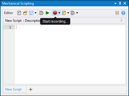
Recording APIs

The Mechanical Scripting pane has a new recording option that enables you to automatically generate or “record” APIs based on the actions you make in the application. In large part, this feature supports the definition of environmental conditions such as contact, loading, and results but can also capture movements made on the model as well as certain display settings and model manipulation features.

mortarboard cap Want to learn more? If you are on Windows, go to the documentation for this topic.
(Requires internet access and will open in a new browser window. Not for Linux platforms.)

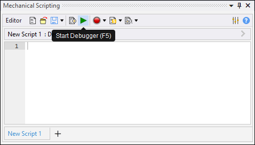
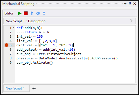
Debugging Scripts and Extensions

The Mechanical Scripting pane also has a new debugging tool. This feature includes tools such as breakpoints, tooltips about variables and script content, a Watch Window to view expressions, and a feature to debug active extensions.

mortarboard cap Want to learn more? If you are on Windows, go to the documentation for this topic.
(Requires internet access and will open in a new browser window. Not for Linux platforms.)

End-to-End API Examples

The Scripting in Mechanical Guide now contains a section dedicated to End-to-End Analysis Examples. These examples provide the API scripts and models required to perform a complete analysis.

mortarboard cap Want to learn more? If you are on Windows, go to the documentation for this topic.
(Requires internet access and will open in a new browser window. Not for Linux platforms.)

Explicit Dynamics

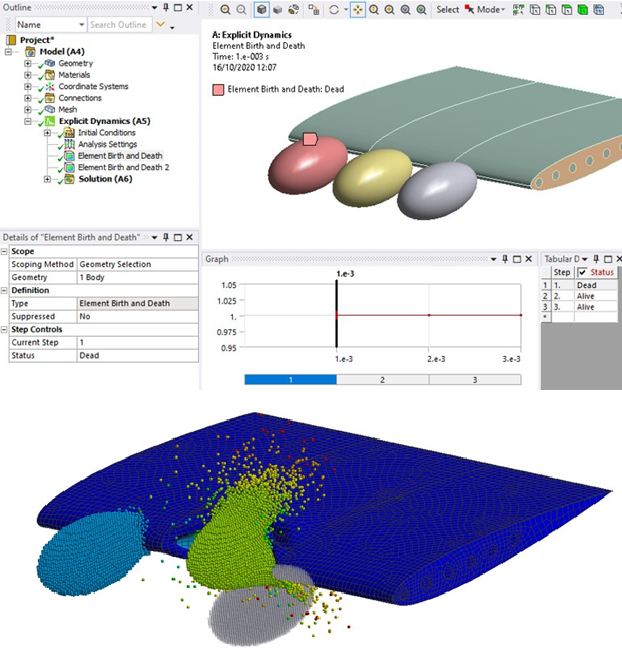
Activation and Deactivation of SPH Bodies

In an Explicit Dynamics Analysis, SPH bodies can be set to inactive for one or more load steps if they are not pertinent to the physical response during those loadsteps using Element Birth and Death objects, which will help to reduce the overall solve time for the model.

mortarboard cap Want to learn more? If you are on Windows, go to the documentation for this topic.
(Requires internet access and will open in a new browser window. Not for Linux platforms.)

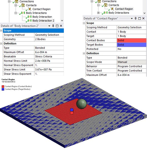
Bonding of SPH to Lagrange Bodies

SPH Bodies can be scoped to Bonded Contact Regions and Bonded Body Interactions to bond them to Lagrange bodies. The bonding enables physically connecting objects of type Lagrange and SPH to benefit from the advantages of both formulations. Bonds can be unbreakable or breakable based on normal or shear Stress criteria.

mortarboard cap Want to learn more? If you are on Windows, go to the documentation for this topic.
(Requires internet access and will open in a new browser window. Not for Linux platforms.)

LS-DYNA

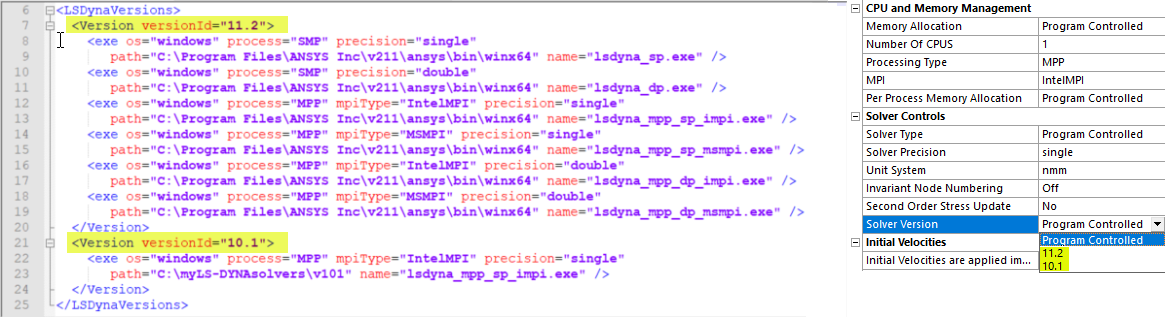
Solver Upgrade and Solver Selection

The default LS-DYNA solver at 2021 R1 is version 11.2. A new feature allows you to use previous versions by defining the versions that are available in a configuration file. Defined versions that match the Precision, Processing, and MPI types will be available in the Solver Version field.

mortarboard cap Want to learn more? If you are on Windows, go to the documentation for this topic.
(Requires internet access and will open in a new browser window. Not for Linux platforms.)

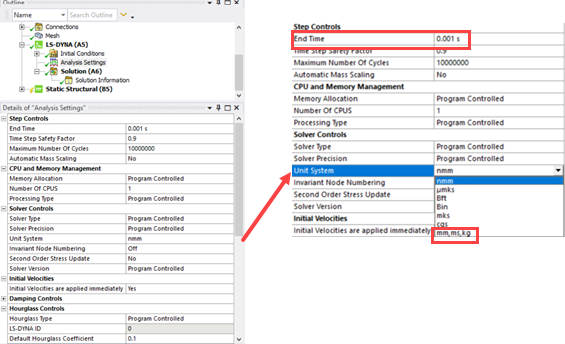
New Unit System (kg, mm, ms, Gpa)

The LS-DYNA extension is now time-aware. Solver Input File is written using this new unit system, and the results are displayed in the GUI defined unit system.

mortarboard cap Want to learn more? If you are on Windows, go to the documentation for this topic.
(Requires internet access and will open in a new browser window. Not for Linux platforms.)

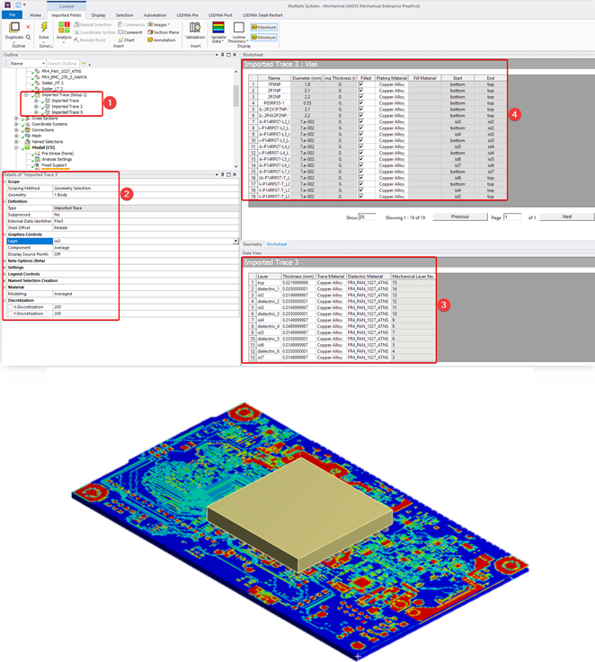
Trace Mapping Support

The LS-DYNA application now supports ECAD trace mapping for structural calculations. Trace mapping is an approach that maps the ECAD information onto the mesh to simplify the modeling.

mortarboard cap Want to learn more? If you are on Windows, go to the documentation for this topic.
(Requires internet access and will open in a new browser window. Not for Linux platforms.)

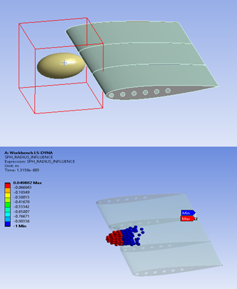
SPH Bounding Box

The calculation domain can now be restricted for SPH particles in the LS-DYNA application. A rectangular box (SPH Box) can be defined to reduce the memory requirements when there are a large number of particles.

mortarboard cap Want to learn more? If you are on Windows, go to the documentation for this topic.
(Requires internet access and will open in a new browser window. Not for Linux platforms.)

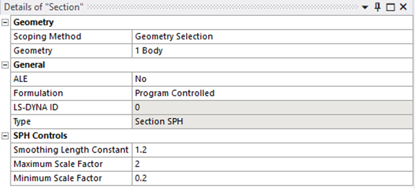
SPH Section Parameters

You can now specify the formulation for the SPH elements in the LS-DYNA application. New SPH Section parameters enable finer control of the simulation.

mortarboard cap Want to learn more? If you are on Windows, go to the documentation for this topic.
(Requires internet access and will open in a new browser window. Not for Linux platforms.)

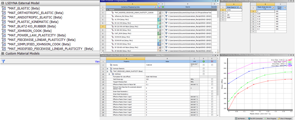
Additional Material Properties

The support of LS-DYNA material models has been enhanced with 10 additional material properties in Engineering Data. These properties are direct equivalents of LS-DYNA material models, with the same names.

mortarboard cap Want to learn more? If you are on Windows, go to the documentation for this topic.
(Requires internet access and will open in a new browser window. Not for Linux platforms.)

Structural Optimization

Calculate Element Pseudo Density

For the Density Based Topology Optimization method, you can now specify a Linear or Non-Linear filter method to calculate the pseudo density of each element. The Linear option enables faster processing as it may prefer placing material on the boundary of your design domain as well as cause the Minimum value of the Member Size property to infringe upon the boundary of the design domain. The Non-Linear (program-controlled default) option uses more advanced algorithms to calculate the pseudo densities that resolve the drawbacks of linear filtering. The following illustrates the difference between the two filters. (The new Filter property is under Analysis Settings.)

Linear

Non-Linear

mortarboard cap Want to learn more? If you are on Windows, go to the documentation for this topic.
(Requires internet access and will open in a new browser window. Not for Linux platforms.)

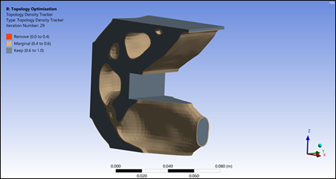
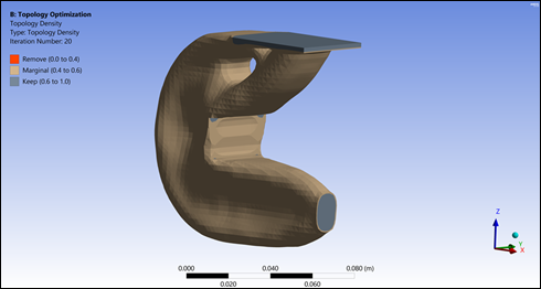
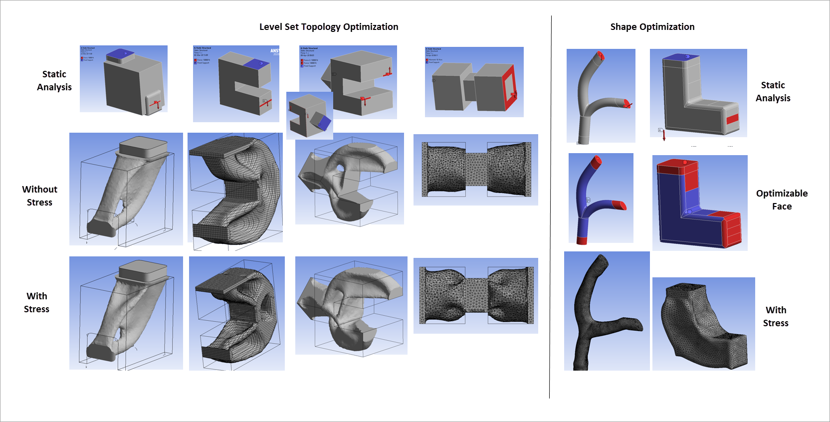
Stress Constraint

You can now use Stress as a Constraint for the Objective object. And, Stress is now supported by the Level Set Topology Optimization method as a Response option as well as an option for the Objective object.

mortarboard cap Want to learn more? If you are on Windows, go to the documentation for this topic.
(Requires internet access and will open in a new browser window. Not for Linux platforms.)

Short Fiber Composites

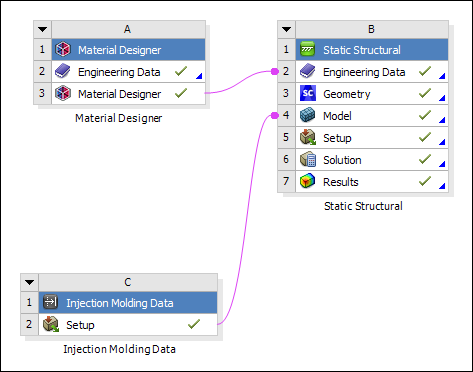
New Workflow

Now, using a new workflow for Short Fiber Composites, you can predict the thermo-mechanical behavior of parts made of short fiber reinforced composites. This workflow combines Material Designer for the material characterization, the new Injection Molding Data system in Workbench that imports injection molding simulation results, and Mechanical for the setup of the finite element model.

mortarboard cap Want to learn more? If you are on Windows, go to the documentation for this topic.
(Requires internet access and will open in a new browser window. Not for Linux platforms.)

ANSYS Motion

Model and Analyze a System of Rigid and/or Flexible Components

The ANSYS Motion system is available in the Analysis Systems toolbox once the ANSYS Motion ACT extension is loaded.

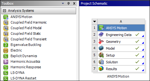
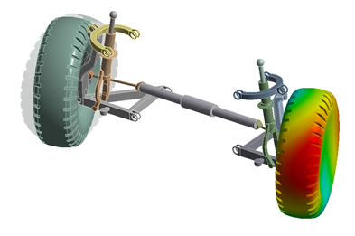
ANSYS Motion allows you to model and analyze the dynamic behavior of a system of interconnected bodies consisting of rigid and/or flexible components.

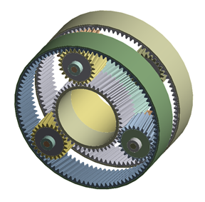
In addition to general features, ANSYS Motion provides the DRIVETRAIN Toolkit that allows you to automate the creation of power transmission device models including gears, bearings, shafts, and housings, and to analyze their dynamic behavior.

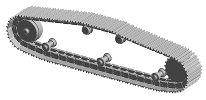
Moreover, the LINKS Toolkit allows you to analyze systems containing flexible power transmission features like chains, tracks, and belts. Connections between the individual links and contact between the links and the sprockets, pulleys, and rollers mean that many hundreds of thousands of elements need to be setup and have their contact defined. In order to realize this, the LINKS Toolkit provides an automated method for quickly setting up these kinds of systems and postprocessing them in an easy manner.

mortarboard cap Want to learn more? If you are on Windows, go to the documentation for this topic.
(Requires internet access and will open in a new browser window. Not for Linux platforms.)

Additive Manufacturing

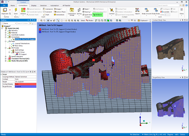
AM Bond

Use the new AM Bond connection when certain mesh and support combinations in Workbench Additive result in a non-contiguous mesh, such as a part meshed with layered tetrahedrons and an STL support meshed with voxels. The internal means of connection is through constraint equations that connect the support nodes to the part elements.

mortarboard cap Want to learn more? If you are on Windows, go to the documentation for this topic.
(Requires internet access and will open in a new browser window. Not for Linux platforms.)