What's New at 2019 R1?
Mechanical Enhancements
Major
Noise, Vibration, and Harshness (NVH) Analysis - Electric Machines
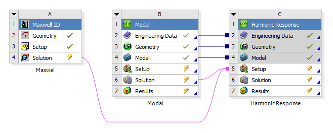
End-to-end simulations of noise and vibration in rotating electric machines are now possible in Release 2019 R1, where coupled workflows between Mechanical and the Maxwell application have been integrated throughout Workbench. You can use Maxwell to calculate the electromagnetic forces developed throughout a range of rotational speeds of the machinery, then transfer those loads to Mechanical by linking the two systems in the Workbench Project Schematic. The downstream Harmonic Response analysis in Mechanical calculates the structural response to those electromagnetic loads over the same rotational speed range.
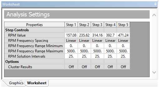
To further support this capability, a new Step Controls category in the Analysis Settings enables you to:
-
Set up a multiple-RPM run where each RPM step has its own response frequency range (minimum and maximum) and frequency spacing.
-
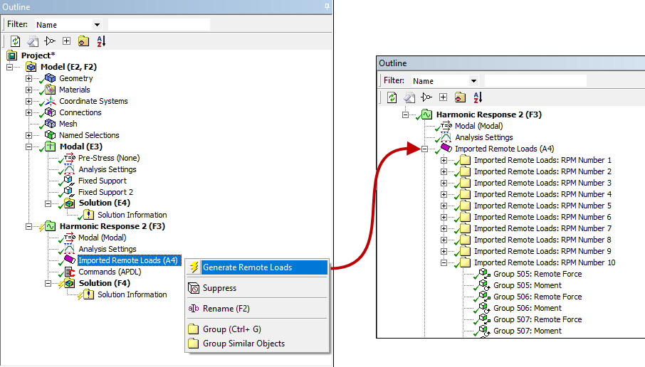
Specify Remote Forces and Moment loading at specific RPM values using the new RPM Varying and RPM Selection properties.

-
Import Remote Force/Moment and Surface Force Density loads from the Maxwell application for one or more RPM loading conditions.
 Want to learn more? If you are on Windows, go to the
documentation for this topic.
Want to learn more? If you are on Windows, go to the
documentation for this topic.
(Requires internet access
and will open in a new browser window. Not for Linux platforms.)
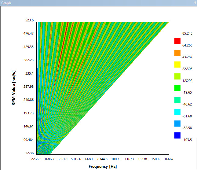
Waterfall Diagram
In the analysis of rotating electric machines, the resultant noise and vibration due to the electromagnetic forces are of primary interest. ANSYS Workbench enables you to evaluate Equivalent Radiated Power (ERP) Waterfall diagrams. ERP diagrams efficiently communicate results that you can use to examine structural vibrations for a range of rotating conditions and frequencies.
Want to learn more? If you are on Windows, go to the
documentation for this topic.
(Requires internet access
and will open in a new browser window. Not for Linux platforms.)
Solution Combination
The capabilities of the Solution Combination feature have been expanded.
New Analysis Types and Multiple Combinations
The Solution Combination feature now supports the combination of the following analysis types. Previously only Static Structural analysis could be combined.
- Harmonic Response
- Static Structural
- Transient Structural
Moreover, you can specify multiple combinations in your simulation. And, each of your base solutions can include a user-defined multiplication coefficient.
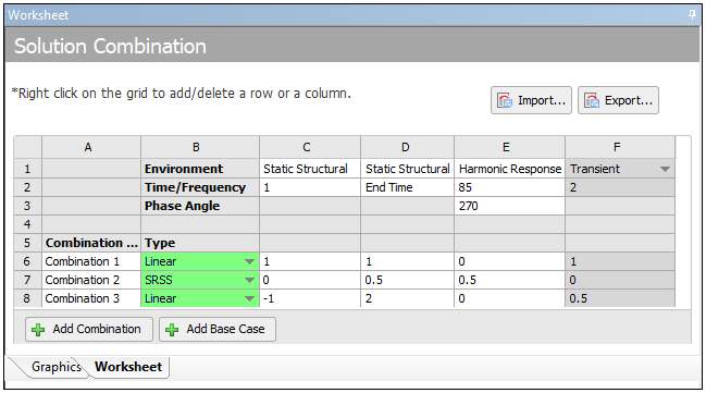
Quadratic (SRSS) Equation Support
As shown in the figure above, you can now specify your solution combinations as either Linear or Quadratic SRSS (Square Root of the Sum of Squares).
Worksheet Redesign
You'll also notice in the above illustration that the Worksheet has been redesigned. Now when you are using the Worksheet, you can set up as many combinations as you wish and define different coefficients and input base cases.
Import and Export Options
Using the Worksheet Export option, you can export the settings that you create as a Comma Separated Value (.csv) file. At that point, you can use any external editor of your choice (such as Microsoft Excel) to modify the .csv data, then import it back to your Mechanical analysis using the Import option.
New Result Display Options
Once you evaluate all of your Solution Combinations, you can pick the combination for which you want to display results using either Tabular Data or a result Set Number.
Want to learn more? If you are on Windows, go to the
documentation for this topic.
(Requires internet access
and will open in a new browser window. Not for Linux platforms.)
Part Transformations
Mechanical now enables you to specify model transformations to modify the position and orientation of the parts in your model. This can be beneficial if you want greater control over the position or location of a part as well as if you wish to simulate different parts orientations.
![]()
![]()
Want to learn more? If you are on Windows, go to the
documentation for this topic.
(Requires internet access
and will open in a new browser window. Not for Linux platforms.)
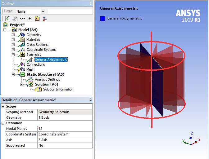
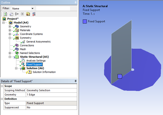
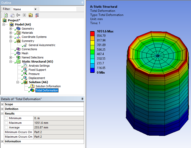
General Axisymmetric
The Symmetry feature offers a new symmetry type for 3D Static Structural analyses: General Axisymmetric. This feature enables you to create a three-dimensional mesh, in the circumferential direction, on a surface body model that is based on specified nodal planes and an axis. This feature supports edge and vertex scoping only. From these surface model edges and vertices, you can generate three-dimensional node-based Named Selections that you can then use as scoping items for other simulation options such as loading conditions and/or results.
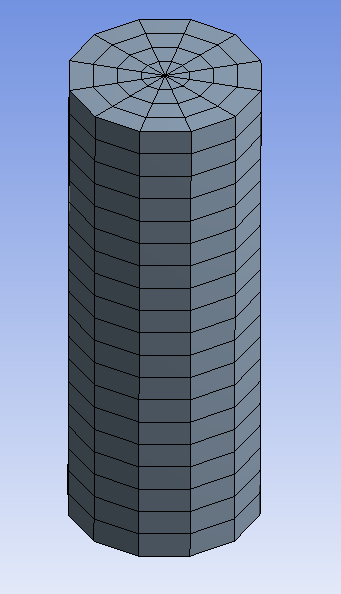
Various models are used to demonstrate some of the General Axisymmetric capabilities in the figures below.
Selected Radial Planes
Generated Mesh
Display of Named Selections
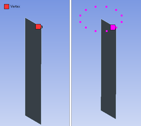
Boundary Condition Scoping
Result Scoping
Element Technology
This feature uses solver element technology based on the elements SOLID272 and SOLID273. The following capabilities are supported for General Axisymmetric:
- The application chooses the node to surface contact detection method when General Axisymmetric bodies are in contact with other bodies.
- Both axisymmetric and non-axisymmetric loads are supported. The Pressure load is applied using Surface Effect elements (SURF159).
Want to learn more? If you are on Windows, go to the
documentation for this topic.
(Requires internet access
and will open in a new browser window. Not for Linux platforms.)
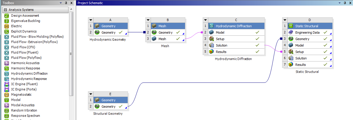
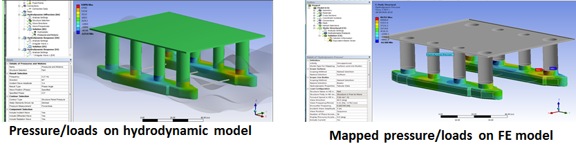
Hydrodynamic Load Transfer from Aqwa
Hydrodynamic Load Mapping ACT Extension
The surface pressures and line loads calculated in a Hydrodynamic Diffraction analysis can now be transferred to panel, solid, and beam elements in a Static Structural analysis using the Hydrodynamic Pressure Mapping ACT extension. This extension replaces a multi-step process and simplifies the load transfer process using a link on the Workbench Project Schematic page. This removes the need to create, manipulate and run files external to Workbench. Multiple wave phase angles can be analyzed in a single Static Structural calculation, to provide a clear picture of finite element results in Mechanical due to hydrodynamic loading over the whole wave cycle.
Hydrodynamic Diffraction -> Static Structural
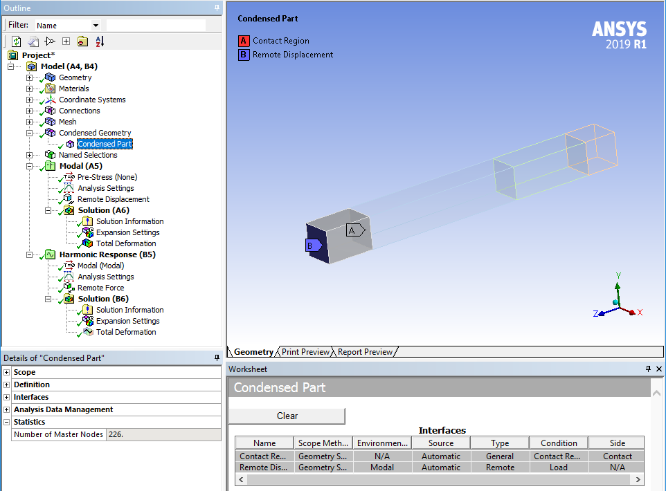
Substructure Analysis (CMS)
For substructure analyses:
- Substructure Analysis using the CMS matrix reduction method is now supported for Harmonic Response analyses based on Mode Superposition (MSUP).
Want to learn more? If you are on Windows, go to the
documentation for this topic.
(Requires internet access
and will open in a new browser window. Not for Linux platforms.)
- The application has a new file management method when you are using the Mechanical APDL Solver. To improve solution processing times and memory usage when solving the Use Pass and Expansion Pass, the application now refers to the prerequisite files generated by the upstream condensed parts using the path to their location instead of making copies of the files.
Want to learn more? If you are on Windows, go to the
documentation for this topic.
(Requires internet access
and will open in a new browser window. Not for Linux platforms.)
Rigid Dynamics On-demand CMS Expansion
CMS expansion allows you to perform expansion on the fly during postprocessing to avoid large RST files with large meshes and/or large number of time points (transient simulation) which are expensive to write/read.
For a medium size model with 14 Condensed Parts, 165867 nodes, 60859 elements, 102 time points, compare the improvement:
- MAPDL expansion: 4m 16s, 14 RST files, total: 3.5 Gb
- On-demand expansion: 22s (deformation + stress), no RST file
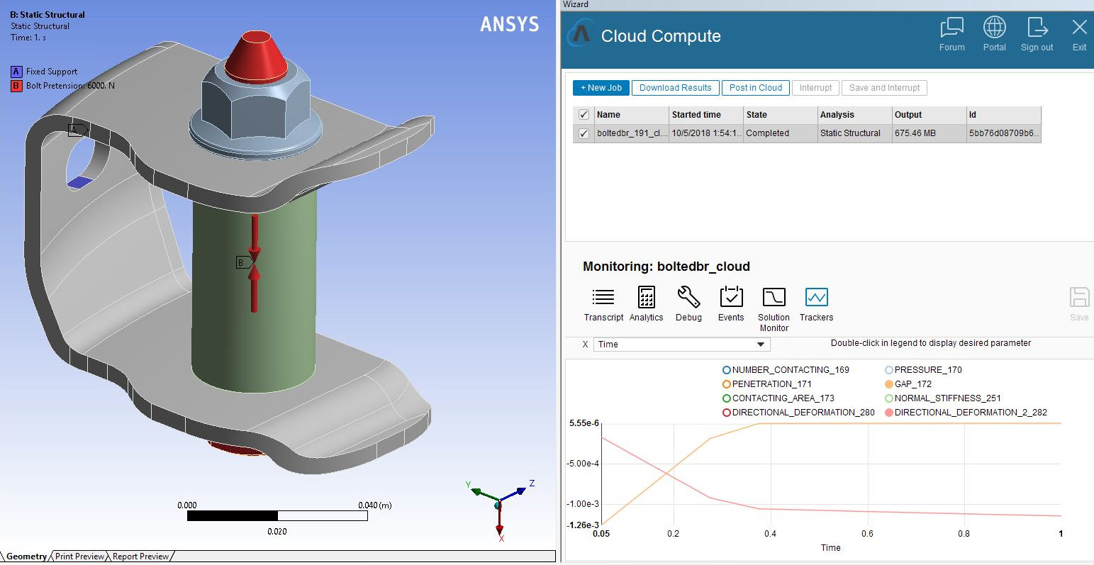
ANSYS Cloud Compute
ANSYS Cloud Compute is a new service that extends the solution capabilities of ANSYS Mechanical and ANSYS Fluent. Cloud Compute allows compute-intensive jobs to be submitted to a multi-core (see below) cloud HPC service managed by ANSYS. Access to the service is provided by a separately installed ACT app. A cloud subscription and a pool of ANSYS Elastic Units (licenses) are required.
- Mechanical jobs can be solved on 12, 36, or 96 cores
- Fluent jobs can be solved on 12, 32, or 112 cores
ANSYS Cloud Compute Dashboard

Setting Up a Cloud Compute Job

Configuring Results Display
Displacement Countours on ANSYS Cloud Compute

Want to learn more? If you are on Windows, go to the
ANSYS
Cloud website
(Requires internet access
and will open in a new browser window. Not for Linux platforms.)
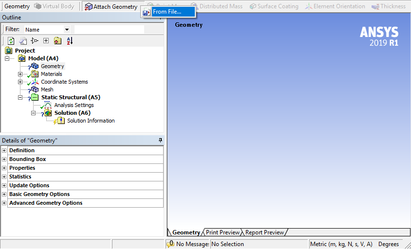
Geometry
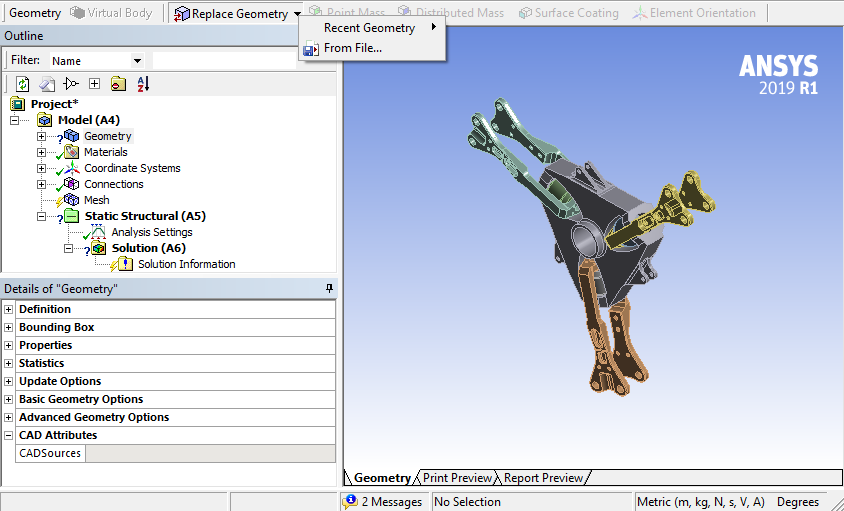
Attach/Replace Geometry
You can now open analysis systems without including a geometry. From Mechanical, the new option Attach Geometry, available from the Geometry object toolbar, enables you to import a geometry from with the application. Once you attach a geometry, or for a system that already includes a geometry, the Replace Geometry option replaces Attach Geometry enabling you to replace an existing geometry.
Want to learn more? If you are on Windows, go to the
documentation for this topic.
(Requires internet access
and will open in a new browser window. Not for Linux platforms.)
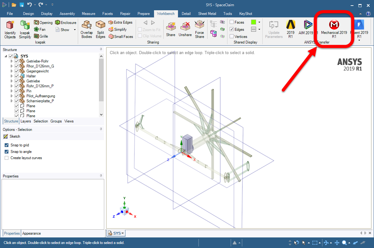
Open Mechanical from Discovery Live and SpaceClaim
The ANSYS Discovery Live and the SpaceClaim applications now include an option to automatically open Mechanical and transfer the active design. The option automatically opens Workbench, places a Mechanical Model system in the Workbench Project Schematic, and then launches the Mechanical application. The Geometry cell of the new Workbench system is associated with the active design in Discovery Live or SpaceClaim.
Meshing
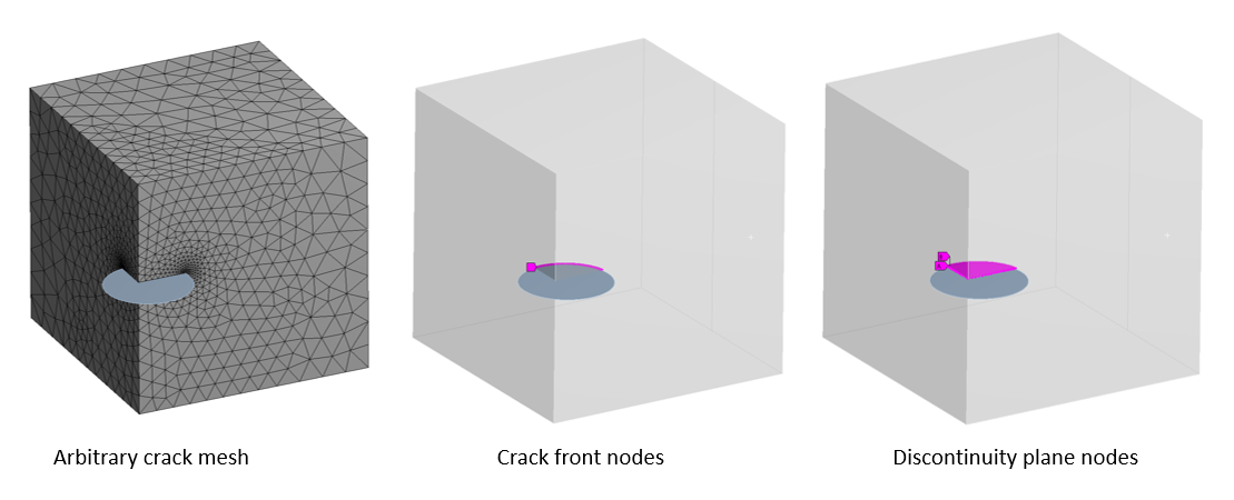
Arbitrary Crack Mesh Generation
An Arbitrary Crack can now span multiple faces and can therefore be used to create corner cracks. Previously, an Arbitrary Crack was confined to one face.
External Model
Cross Section Transverse Shear Stiffness
For imported line body meshes, if included in your source file, External Model enables you to import Transverse Shear Stiffness XY and Transverse Shear Stiffness XZ as cross section object data.
Want to learn more? If you are on Windows, go to the
documentation for this topic.
(Requires internet access
and will open in a new browser window. Not for Linux platforms.)
Element FLUID116 Support
The External Model system now enables you to import the link element FLUID116 into Mechanical from Mechanical APDL common database (.cdb) files.
Want to learn more? If you are on Windows, go to the
documentation for this topic.
(Requires internet access
and will open in a new browser window. Not for Linux platforms.)
Connections
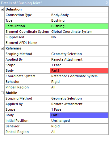
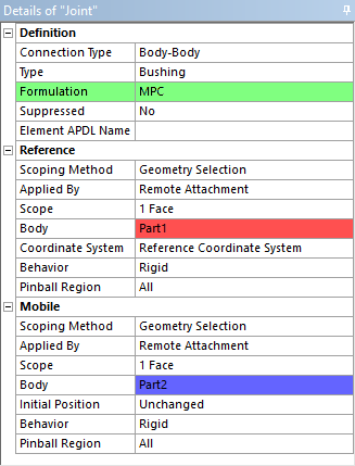
Bushing Joint
The Bushing Joint has a new element definition property: Formulation, which has been added to support Bushing Formulation. Now, using the new property, you can select MPC or the new Bushing formulation. The Bushing formulation uses the COMBI250 element and is currently only supported for Modal and Harmonic Analysis types. In previous releases, the application always used the MPC (Multi-Point Constraint) formulation for Bushing joints.
Want to learn more? If you are on Windows, go to the
documentation for this topic.
(Requires internet access
and will open in a new browser window. Not for Linux platforms.)
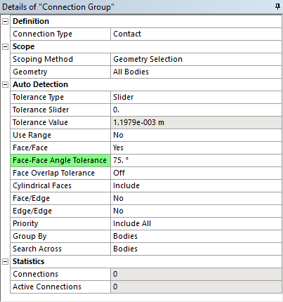
Contact Detection for Faces
The Connection Group object has a new property: Face/Face Angle Tolerance. When working with Face/Face automatic contact detection, this property enables you to define the minimum angle between two face normals. This minimum angle is the threshold below which the application will ignore the faces from proximity detection. The default value is 75°, the minimum value is 0°, and the maximum value is 90° (perpendicular).
Want to learn more? If you are on Windows, go to the
documentation for this topic.
(Requires internet access
and will open in a new browser window. Not for Linux platforms.)
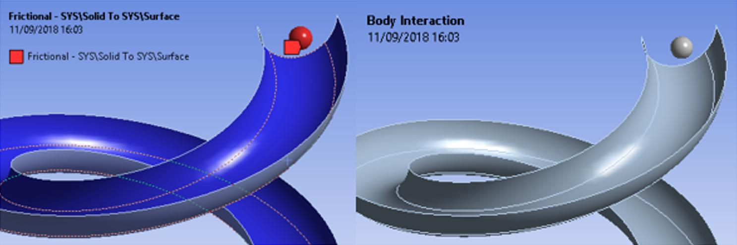
Manual Contact Treatment for Explicit Dynamics
A new option exists which allows more refined definition of contact regions in Explicit Dynamics. By setting the Manual Contact Treatment option to Pairwise, Contact Regions are treated individually. This is in contrast to the original behavior (which is obtained by setting the Manual Contact Treatment to Lumped) where all surfaces allocated to any Contact Region are added to a collective pool of surfaces that could interact with each other via contact. This allows for better control of the definition of friction coefficients between surfaces. Additionally, the symmetry behavior is now respected when using the Pairwise Manual Contact Treatment option, and additional scoping options for the Contact and Target regions are now available.
- Friction definition is applied per contact pair
- Scoping:
- Contact region: nodes in contact
- Target region: faces in contact
Analyses
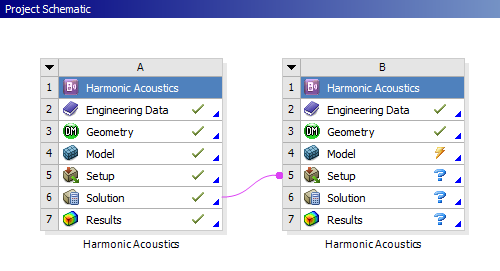
Harmonic Acoustics Analyses
You can now perform one-way vibro-acoustic coupling between FSI Harmonic Acoustics analysis and a Harmonic Acoustics analysis.
Want to learn more? If you are on Windows, go to the
documentation for this topic.
(Requires internet access
and will open in a new browser window. Not for Linux platforms.)
Topology Optimization Analyses
The following new capabilities and features are available when performing a Topology Optimization analysis.
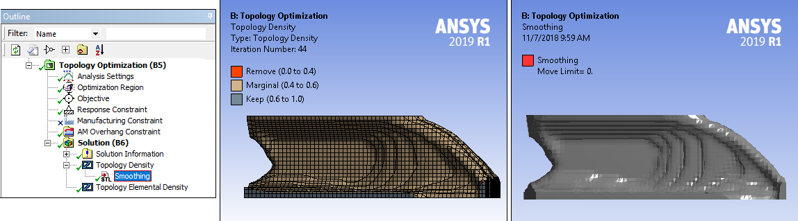
Smoothing Result
The Topology Optimization has a new object: the Smoothing object. You add this object from a Topology Density result. It enables you to create a smoothed geometry based on the parent Topology Density result. Furthermore, the application automatically creates an STL (Stereolithography) geometry file of the smoothed geometry. You can smooth any number of parts on your model.
Steady-State Thermal Support
You can now optimize an upstream Steady-State Thermal system. In addition, for this newly supported upstream analysis type:
- Thermal Compliance is available as a Response Type in the Objective object Worksheet for the Mass and Volume Response Constraints.
- There is a new Response Constraint type: Temperature. This Temperature constraint enables you to put an upper bound on the temperatures at the nodes corresponding to the selection.
Local von-Mises Stress Constraint
The scoping for the Local von-Mises Stress Constraint is no longer restricted to the elements in the Optimization Region. You can now scope this to any region of your model.
Shell Body Support
The Topology Optimization analysis now supports shell bodies used in upstream Static Structural, Modal, and Steady-State Thermal systems.
Reload Volume Fraction from a Solved Iteration
The Topology Optimization analysis has a new Analysis Settings category: Reload Volume Analysis. Once you have completed the solution process for your analysis, this category displays. The category, and its properties, Reload Volume Fraction and Current Reload Point, enable you to load a previous solution point as a starting point for your next desired solution.
Want to learn more? If you are on Windows, go to the
documentation for this topic.
(Requires internet access
and will open in a new browser window. Not for Linux platforms.)
Additive Manufacturing (AM) Analyses
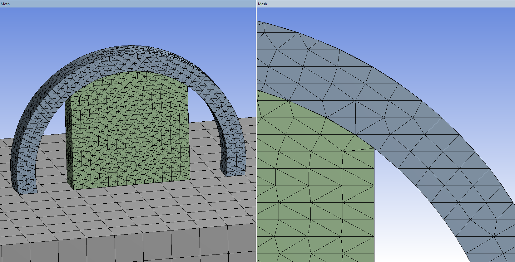
Layered Tetrahedrons Mesh
A new Layered Tetrahedrons Mesher creates a tetrahedrons mesh that conforms to a specified layer size. It captures geometry well, and is useful if your part has small features, such as holes, or for thin-walled parts and supports.
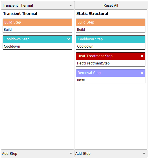
Heat Treatment
You can now simulate heat treatment following the build process using a new Heat Treatment Step on the AM Process Sequencer. For example, you may wish to capture an annealing process by specifying a Relaxation Temperature in Analysis Settings or by specifying creep properties in Engineering Data.
New Materials
Two new sample materials have been added to the Additive Manufacturing Materials library, 17-4PH Stainless Steel and AlSi10Mg.
Other Enhancements
- You can now specify model transformations to modify the position and orientation of the parts in your build. This can be beneficial if you want greater control over the position or location of a part or if you want to simulate different part orientations.
- The application now supports Restarts during AM Process Simulations.
- You can now model powder between and around parts using an ANSYS-defined named selection, POWDER_ELEMENTS (an elements component).
- You can now model components above the build plate that are not being 3D printed, such as clamps, measuring devices, and instrumentation using an ANSYS-defined named selection, NONBUILD_ELEMENTS (an elements component). These non-build items may influence heat dissipation and/or part distortion.
Want to learn more? If you are on Windows, go to the
documentation for this topic.
(Requires internet access
and will open in a new browser window. Not for Linux platforms.)
Material-Dependent Damping
The material-dependent damping property Constant Structural Damping Coefficient, from the Engineering Data Workspace, is now supported for Full transient, Full Harmonic Response, Full Damped Modal, and Reduced Damped Modal analyses (when the Store Complex Solution property is set to Yes.
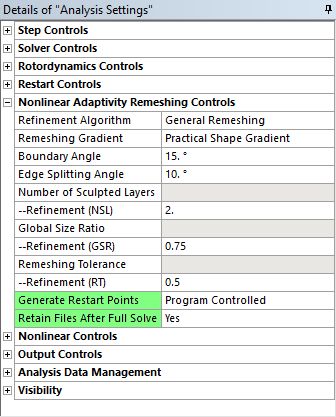
Nonlinear Adaptivity Remeshing Controls
Now, when you are using the Nonlinear Adaptive Region condition, there are two new properties in the Nonlinear Adaptivity Remeshing Controls category of the Analysis Settings: Generate Restart Points and Retain Files After Full Solve. These properties enable you to control whether restart points are created and whether you want to save the associated files following the solution process.
Want to learn more? If you are on Windows, go to the
documentation for this topic.
(Requires internet access
and will open in a new browser window. Not for Linux platforms.)
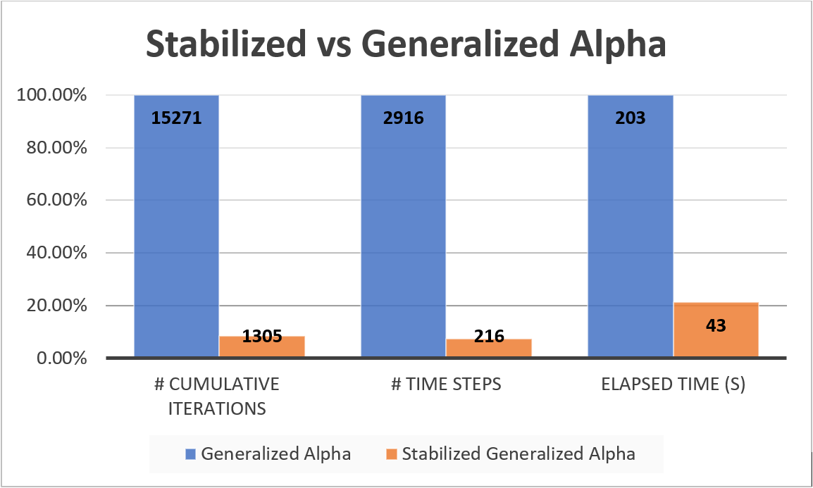
Rigid Dynamics Stabilized Generalized Alpha Time Integration
New Stabilized Generalized Alpha time integration enforces constraints while preserving dynamic equilibrium with no spurious oscillation, faster convergence and larger time steps.
Loading
Convection Fluid Flow
The Convection boundary condition now supports vertex and node scoping when using information from Thermal Fluid line bodies. This feature enables you to use a specific vertex or node to get the bulk temperature in the convection calculations.
Want to learn more? If you are on Windows, go to the
documentation for this topic.
(Requires internet access
and will open in a new browser window. Not for Linux platforms.)
Scripting
Mechanical Scripting
There are several new or updated capabilities available in Mechanical Scripting, including:
- Interacting with details view properties, including parameterization
- Camera manipulation
- Export of graphics (image and 3D models)
- Section Planes
- Returning values from JScript to Python
Want to learn more? If you are on Windows, go to the
documentation for this topic.
(Requires internet access
and will open in a new browser window. Not for Linux platforms.)
Solution and Results
Participation Factor Summary
When you specify the Participation Factor Summary option for the Solution Output property, an associated property, Summary Type, is displayed. For this property, the option Ratio of Effective Mass to Total Mass now supports 2D analyses. It previously only supported 3D analyses.
Want to learn more? If you are on Windows, go to the
documentation for this topic.
(Requires internet access
and will open in a new browser window. Not for Linux platforms.)
Fatigue Results
You can now export the Fatigue graph results Rainflow Matrix and Damage Matrix as a text file.
Want to learn more? If you are on Windows, go to the
documentation for this topic.
(Requires internet access
and will open in a new browser window. Not for Linux platforms.)
New Energy Probes and Energy Trackers for Explicit Dynamics
All new Energy Probes (Internal, Kinetic, Plastic Work, Hourglass, Contact, Total) and two new Energy Trackers (Hourglass, Contact) are available for Explicit Dynamics analyses.
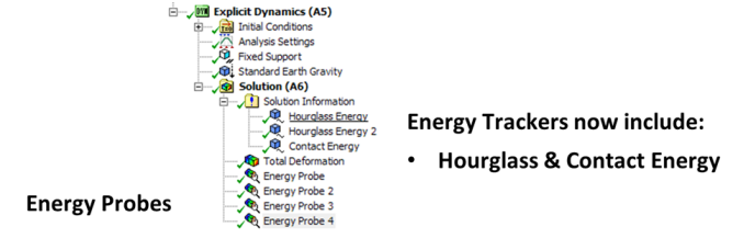
- Energy Probes can be added after the solve
- Energy Trackers are defined before the solve
Graphical
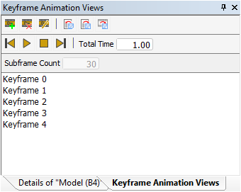
Keyframe Animation
Mechanical now offers a Keyframe animation feature that enables you to string together snapshots of your model in the Geometry window to create an animation. Each Keyframe is a Start and End point that the application then links together by drawing Subframes to create the animation. The application interpolates the transition from keyframe to keyframe to create a smooth animation. For example, you can create an animation of your model rotating. The Keyframe Animation window and an exported GIF file as illustrated below.
Want to learn more? If you are on Windows, go to the
documentation for this topic.
(Requires internet access
and will open in a new browser window. Not for Linux platforms.)
Animation Improvements
The Animation feature has new export capabilities, including:
- When exporting an animation, the application applies the settings of the number of frames and the setting of the time to the exported file. In previous releases, the frame count and timing were based on application defaults.
- The Export feature now supports the GIF file format.
- You can animate a result based on predefined Keyframe Animations as well as synchronize the result's animation to the predefined keyframes.
- You can now export animations on the Linux platform.
Want to learn more? If you are on Windows, go to the
documentation for this topic.
(Requires internet access
and will open in a new browser window. Not for Linux platforms.)
Ease-of-Use
Simulation Templates
You can now create simulation templates in Mechanical. This capability enables you to quickly reuse a setup for different geometries. You can open the application without attaching a geometry and define criterion-based Named Selections that you can then scope to many different analysis objects. Once you define analysis conditions, you can save the project and use the setup for any desired model. The project becomes a template for an analysis.
Want to learn more? If you are on Windows, go to the
documentation for this topic.
(Requires internet access
and will open in a new browser window. Not for Linux platforms.)
Solution Information Worksheet
Now, when you display the Solver Output from the Solution Information object following the solution process, and you scroll through Worksheet content, the application saves the scroll position. As you navigate to another object in the project and return to the Worksheet, the previous scroll position is still active. Previously, the application would redisplay content from the top of the Worksheet.
Want to learn more? If you are on Windows, go to the
documentation for this topic.
(Requires internet access
and will open in a new browser window. Not for Linux platforms.)
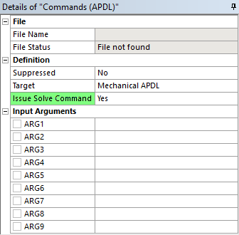
Commands (APDL) Object
The Commands (APDL) object has a new property: Issue Solve Command. This property is only available for a Commands (APDL) object inserted under the Environment of a simulation that uses the Mechanical APDL solver. It enables you to specify whether to solve a load step (or steps).
Want to learn more? If you are on Windows, go to the
documentation for this topic.
(Requires internet access
and will open in a new browser window. Not for Linux platforms.)
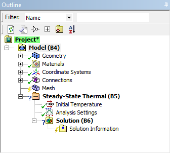
Project Object
The Project object in the Outline now displays with an asterisk (*) in its name to indicate that you have not yet saved the Mechanical database since the last change or set of changes.
Want to learn more? If you are on Windows, go to the
documentation for this topic.
(Requires internet access
and will open in a new browser window. Not for Linux platforms.)
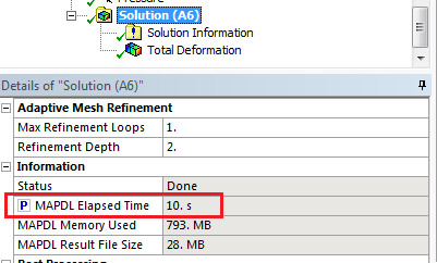
Parameterization of "Elapsed Time"
On the Solution object, the Elapsed Time value can now be parameterized.
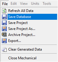
Quickly Save Mechanical Session
A new File menu option is available: Save Database. This option enables you to save the current Mechanical session without having to save the entire project. However, you must save the project when you exit the application to properly save your changes.
Want to learn more? If you are on Windows, go to the
documentation for this topic.
(Requires internet access
and will open in a new browser window. Not for Linux platforms.)
Analysis Settings Worksheet for Rigid Dynamics and Explicit Dynamics
A new Analysis Settings worksheet is available to review step-aware settings.
Korean, Japanese, and Chinese Character Support in File and Folder Names
Previously, Mechanical jobs that tried to run the Mechanical APDL solver in a folder named with Korean, Japanese, or Chinese characters would fail because the solver did not support those characters in file and folder (directory) names. That support has now been added to the solver, therefore those Mechanical jobs are possible at Release 2019 R1.
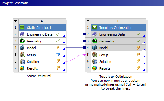
Project Naming in Workbench
As illustrated below, you can now create multi-line names for your project. Use the key combination [Ctrl] + [Enter] to break the lines as desired.