
Major Efforts
Chaining Remote Points
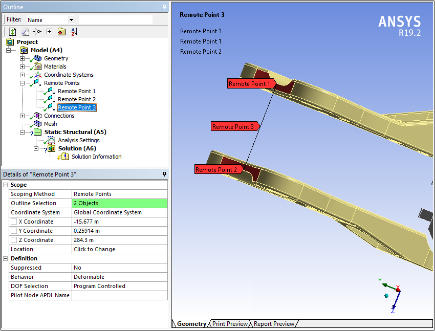
At 19.2, the Remote Point object has new scoping options: Remote Points and Remote Points and Nodes. Using these options, you can scope a remote point to one or more other remote points, as well as nodes...
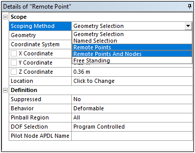
...thereby chaining the Remote Points together. As illustrated in this example, Remote Point 3 is scoped to Remote Points 1 and 2 and its location is defined accordingly.
 Want to learn more? If you are on Windows, go to the
documentation for this item by clicking
here
Want to learn more? If you are on Windows, go to the
documentation for this item by clicking
here
(Requires internet access and will open in a new browser window. Not for Linux platforms.)
Topology Optimization Analysis
Topology Optimization Analysis has a number of new capabilities.
Topology Optimization — Linux Support
Topology Optimization is now supported on the Linux platform. All topology features and options are supported, except Geometry modifications for Design Validation (this requires SpaceClaim, which is not supported on the Linux platform).
Topology Optimization — Lattice Optimization
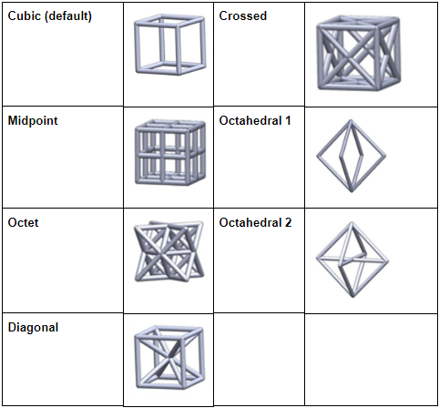
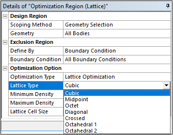
You can now create lightweight parts using optimized lattice structures. The supported lattice types are shown here:
The Optimization Region object, as shown here, provides this new Lattice Optimization option.
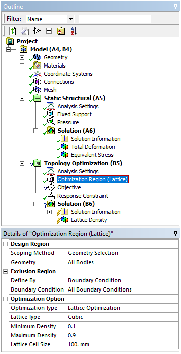
Once the Lattice Optimization type is specified, you select the Lattice Type from the seven supported types.
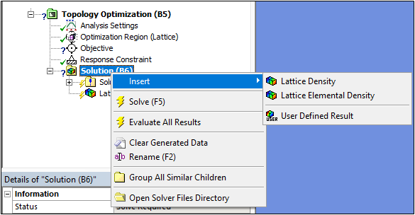
Similar to Topology Optimization analyses, Mechanical automatically inserts density result objects. Supported lattice results include Lattice Density and Lattice Elemental Density:
Want to learn more? If you are on Windows, go to the
documentation for this item by clicking
here
(Requires internet access and will open in a new browser window. Not for Linux platforms.)
Topology Optimization — Additive Manufacturing
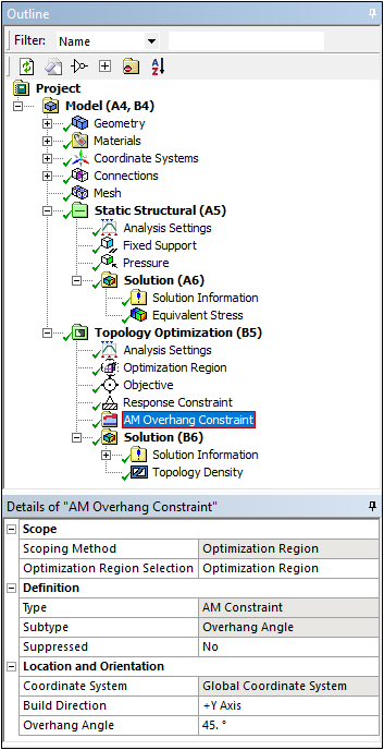
The Topology Optimization analysis has a new additive manufacturing-based constraint option: AM Overhang Constraint. This constraint enables you to eliminate the use of supports for additive printing for a specified Overhang Angle and Build Direction:
Want to learn more? If you are on Windows, go to the
documentation for this item by clicking
here
(Requires internet access and will open in a new browser window. Not for Linux platforms.)
Topology Optimization — Loading Conditions
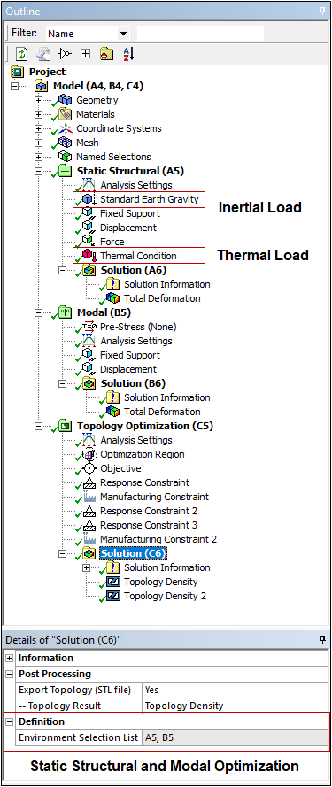
As you can see here, Topology Optimization now supports Inertial and Thermal loads for a Static Structural analysis in combination with a Modal analysis.
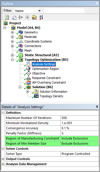
Topology Optimization — Analysis Settings
The Topology Optimization Analysis has two new Analysis Settings properties:
- Region of Manufacturing Constraint: This property enables you to specify to Include (default) or Exclude Exclusions. This feature supports the Pull Out Direction, Extrusion, Cyclic, and Symmetry Manufacturing Constraint options. Selecting Include Exclusions satisfies the constraints for the Exclusion Region.
- Region of Min Member Size: This property enables you to specify to Include or Exclude Exclusions (default). Selecting Exclude Exclusions satisfies the Minimum Member Size for the Exclusion Region.
Want to learn more? If you are on Windows, go to the
documentation for this item by clicking
here
(Requires internet access and will open in a new browser window. Not for Linux platforms.)
Substructuring
There are three additions of note for Substructuring.
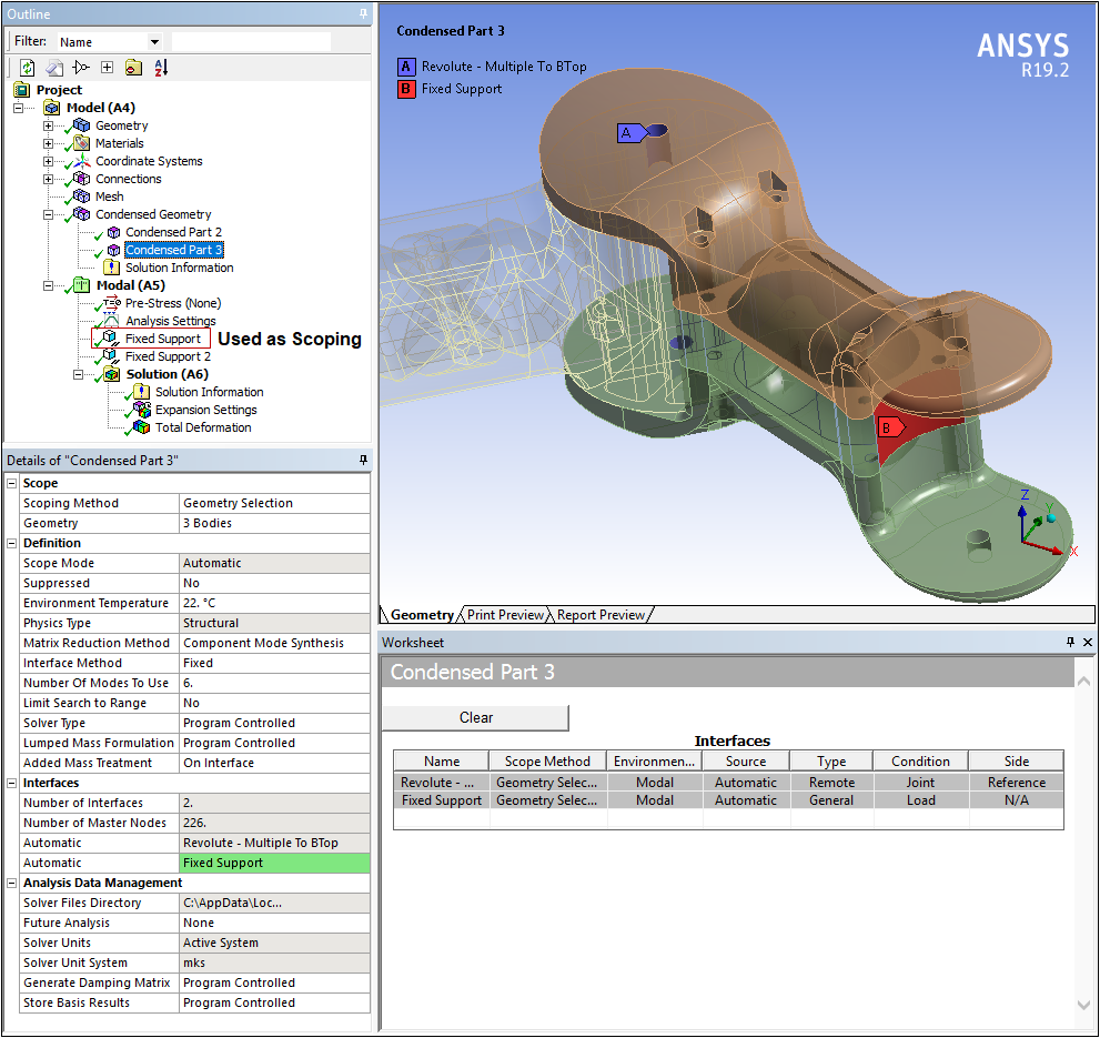
Substructuring — Modal Analysis Support
The Substructuring feature now supports Modal analysis. When using the feature with a Modal analysis, the application can automatically detect all boundary conditions (as illustrated below) that exists in the analysis as Condensed Part Interfaces. This includes Joints, Springs, Bearings, Contacts, Remote Points. In addition, you can manually add node-based named selections to these interfaces. Furthermore, you can define the Solver Type as Direct, Supernode, or Subspace. Lumped Mass formulation is also supported and Mass Treatment is now supported for both Point Mass and Distributed Mass.
Want to learn more? If you are on Windows, go to the
documentation for this item by clicking
here
(Requires internet access and will open in a new browser window. Not for Linux platforms.)
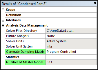
Substructuring — Condensed Part Properties
The Condensed Part object includes three new properties, as illustrated in the Details view example below.
- Generate Damping Matrix: This property enables you to include or exclude damping effects.
- Statistics: This property lists the number of master nodes used for the Generation Pass. This value differs from the value shown for the Number of Master Nodes property of the Interfaces category, whose nodes are modified and the Generate Condensed Part action is not executed.
Want to learn more? If you are on Windows, go to the
documentation for this item by clicking
here
(Requires internet access and will open in a new browser window. Not for Linux platforms.)
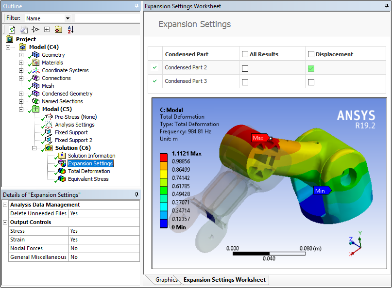
Substructuring — Expansion Pass Worksheet
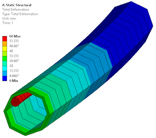
The new Expansion Pass Worksheet displays once you solve your substructuring analysis and select the Expansion Settings object. With this new Worksheet, you specify the condensed parts for which you want to compute results (Displacement or All Results, including stress and strain). To actually display these results, you must also make the data available in the results file by setting the corresponding Output Controls properties in the Details view to Yes. The properties you can control individually include Stress, Strain, Nodal Forces, and General Miscellaneous. By default, the Stress and Strain properties are set to Yes. If none of these Output Controls properties is active (set to Yes), condensed part results will not display in the Geometry window.
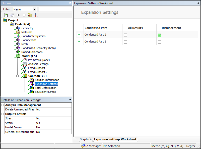
The following example shows Displacement selected for Condensed Part 2 in the worksheet, but not for Condensed Part 3. Looking at the Total Deformation result, we can see the displacement of Condensed Part 2, but not Condensed Part 3.
Want to learn more? If you are on Windows, go to the
documentation for this item by clicking
here
(Requires internet access and will open in a new browser window. Not for Linux platforms.)
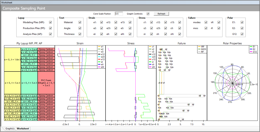
Composite Sampling Point
The new Composite Sampling Point object enables you to plot composite part result data. The feature displays the through-the-thickness result distribution in the laminate for selected points.
Want to learn more? If you are on Windows, go to the
documentation for this item by clicking
here
(Requires internet access and will open in a new browser window. Not for Linux platforms.)
Physics Enhancements
External Model
External Model — Geometry Synthesis Options
The External Model system has a new Project page property (Create Geometry) that enables you to choose whether or not to create geometry from your mesh file. The following examples show a generated geometry as well as an element-based mesh.
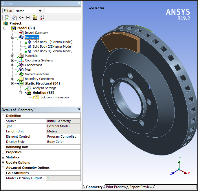
Imported Solid Geometry
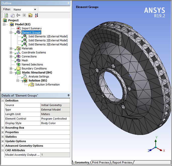
Imported Element-Based Mesh
Only importing the mesh can dramatically decrease import time and significantly reduce the amount of memory used during the process.
Want to learn more? If you are on Windows, go to the
documentation for this item by clicking
here
(Requires internet access and will open in a new browser window. Not for Linux platforms.)
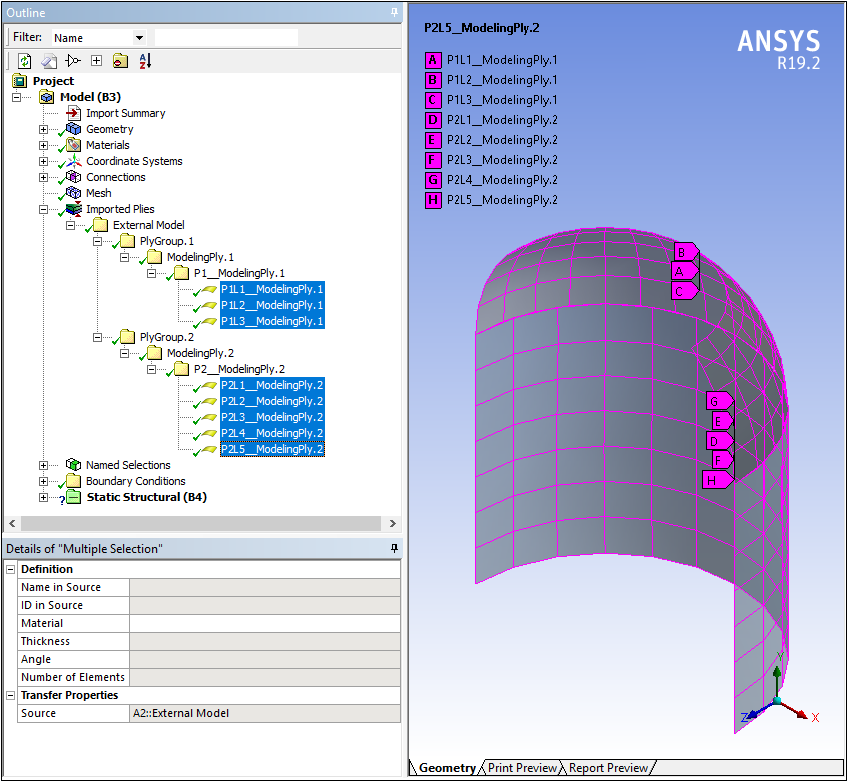
External Model — Importing Composite Data
You can now import composite ply data from Mechanical APDL (.cdb) and NASTRAN Bulk Data (.bdf, .dat, .nas) files.
Want to learn more? If you are on Windows, go to the
documentation for this item by clicking
here
(Requires internet access and will open in a new browser window. Not for Linux platforms.)
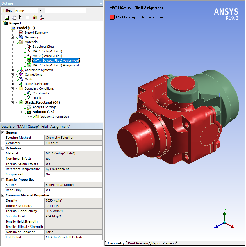
External Model — Automatic Material Assignment
Now, whenever multiple bodies in your upstream mesh file are assigned the same materials, the application automatically creates a Material Assignment object for the associated bodies. This makes sure that each body has the same unique material identifier.
Want to learn more? If you are on Windows, go to the
documentation for this item by clicking
here
(Requires internet access and will open in a new browser window. Not for Linux platforms.)
External Model — Importing Load Data
The External Model system now supports the import of:
- Thermal convection and heat flux loads as surface loads from Mechanical APDL (.cdb) and Abaqus Input (.inp) files. You can also specify Convection and Heat Flux on imported Surface Load boundary conditions.
- Gravity boundary conditions, in the form of an Acceleration object, for Mechanical APDL (.cdb), Abaqus Input (.inp), and Nastran Bulk Data (.bdf, .dat, .nas) files.
Want to learn more? If you are on Windows, go to the
documentation for this item by clicking
here
(Requires internet access and will open in a new browser window. Not for Linux platforms.)
External Model — Promotion
You can now promote Connections to Remote Points. For imported Flexible Remote Connectors and/or Rigid Remote Connectors, you can automatically create a Remote Point object from Worksheet that you can then use to scope other objects.
External Model — ACT Extension
You can now access NASTRAN mesh-based databases through ACT extensions and console window.
Acoustics Analysis
Acoustics Analysis — Prestressed Harmonic Acoustics Analysis
Mechanical now enables you to perform a Fluid Structure Interface (FSI) Harmonic analysis using a prestressed structure from a Static Acoustics Analysis. This simulation supports all acoustic boundary conditions and loads that are defined in the downstream system, except the Absorbing Element boundary condition and the Transfer Admittance Matrix and Low Reduced Frequency Model Acoustic Models. All results options are supported.
Want to learn more? If you are on Windows, go to the
documentation for this item by clicking
here
(Requires internet access and will open in a new browser window. Not for Linux platforms.)
Acoustics Analysis — FSI Cyclic Symmetry
As illustrated by the example result below, Mechanical now supports Cyclic Symmetry and Premeshed Cyclic Symmetry regions for all acoustics-based analysis systems: Harmonic, Prestressed Harmonic, Modal, Prestressed Modal, and Static.
Want to learn more? If you are on Windows, go to the
documentation for this item by clicking
here
(Requires internet access and will open in a new browser window. Not for Linux platforms.)
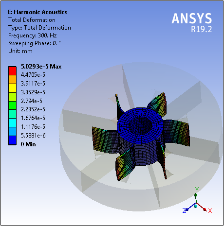
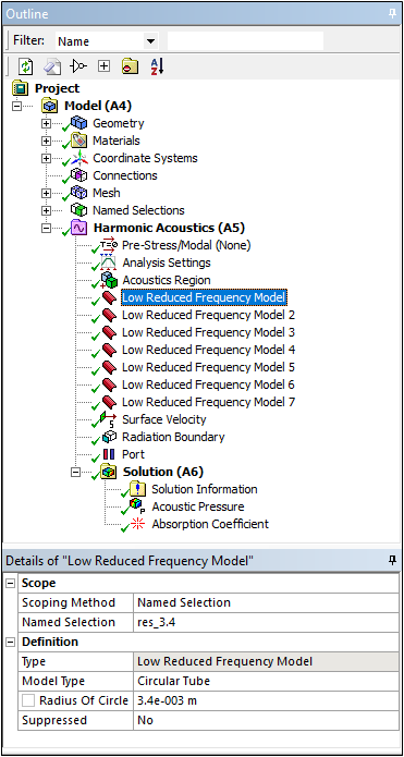
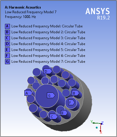
Acoustics Analysis — Low Reduced Frequency Model
Harmonic Acoustics and Structural Acoustics analyses support a new Acoustic Model: Low Reduced Frequency. With this model, for specific structures you can account for the interaction between an acoustic pressure wave in a viscous fluid and a rigid wall, according to a Low Reduced Frequency (LRF) approximation.
Want to learn more? If you are on Windows, go to the
documentation for this item by clicking
here
(Requires internet access and will open in a new browser window. Not for Linux platforms.)
Ease of Use Enhancements
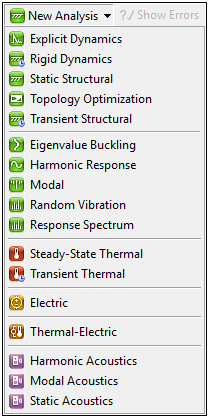
Adding New Analyses from Within Mechanical
The New Analysis drop-down menu on the Standard Toolbar includes all the available Mechanical analysis types. When you add a new system through this menu, the Project Schematic automatically updates.
Linking Analysis Systems
Mechanical now enables you to link and unlink analysis systems, such as Thermal-Stress or Prestressed Modal, from within the application without having to return to the Project Schematic. This new capability automatically creates or deletes the links between the corresponding systems in the Workbench Project Schematic. This feature supports all linked analyses.
Preference Migration
Most ANSYS Workbench preferences are now automatically migrated when you install a new version of the application. This includes licensing settings, Options panel settings, solver preferences, and Engineering Data settings.
Want to learn more? If you are on Windows, go to the
documentation for this item by clicking
here
(Requires internet access and will open in a new browser window. Not for Linux platforms.)
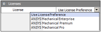
License Selection
A new category and property has been added for the Model cell when selected in the Workbench Project Schematic. The new property, License, enables you to specify the license that will be used by a new instance of the Mechanical application for your model.
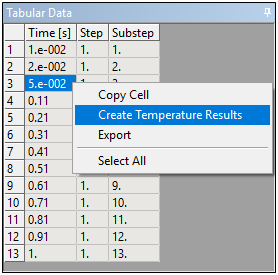
Create Temperature Results from Tabular Data Window
For thermal analyses, Mechanical now provides the context menu option Create Temperature Results on the Tabular Data of the Solution folder and it enables you to automatically create multiple temperature results based on the selected rows of the Tabular Data window.
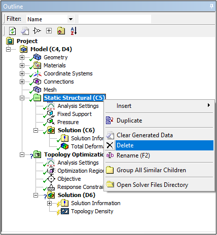
Delete an Environment
You can now delete environments from within the Mechanical application if your Model includes more than one environment. This action also removes the corresponding system from the Workbench Project Schematic.
Want to learn more? If you are on Windows, go to the
documentation for this item by clicking
here
(Requires internet access and will open in a new browser window. Not for Linux platforms.)
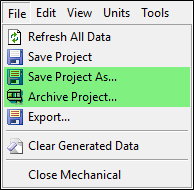
Saving and Archiving Projects
Mechanical now has the file menu options Save Project As and Archive Project.
Want to learn more? If you are on Windows, go to the
documentation for this item by clicking
here
(Requires internet access and will open in a new browser window. Not for Linux platforms.)
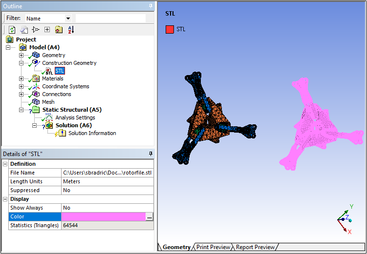
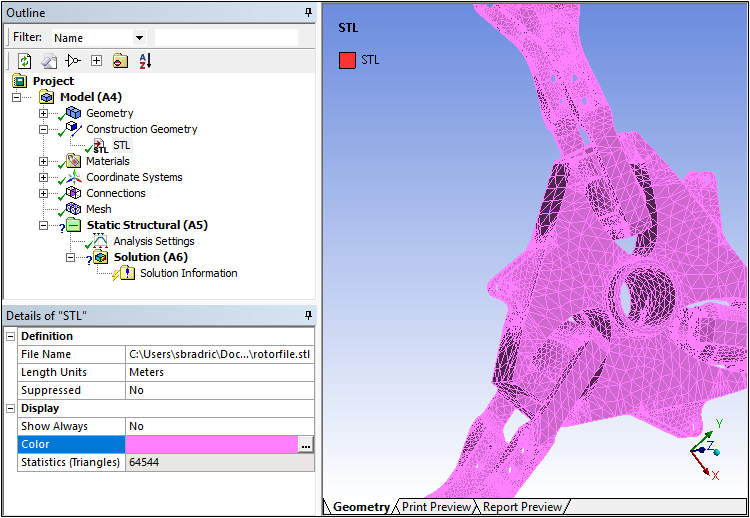
Import STL as Construction Geometry
The new Construction Geometry option, STL, enables you to import and view an STL file in your simulation. In addition, you can export your existing model as an STL file and then import it, as shown in the following example.
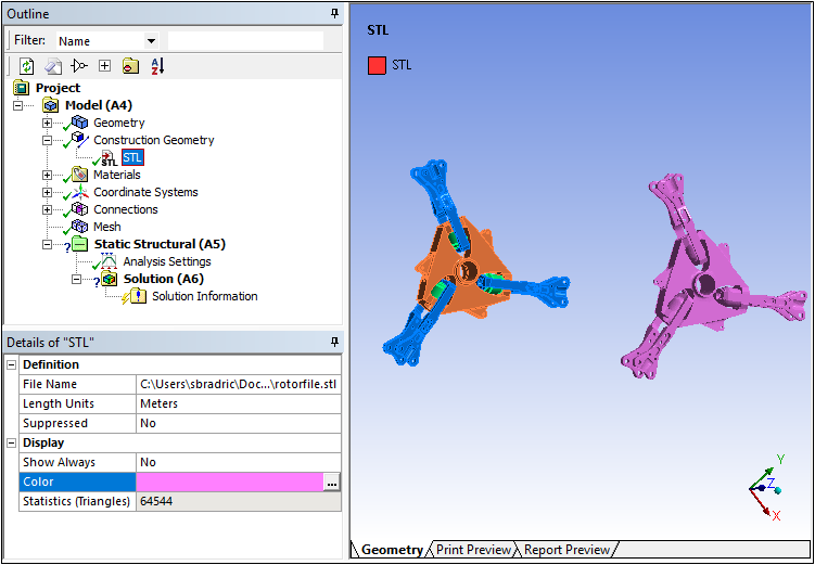
Once imported, you can mesh the imported STL model (as well as your original model).
Want to learn more? If you are on Windows, go to the
documentation for this item by clicking
here
(Requires internet access and will open in a new browser window. Not for Linux platforms.)
Boundary Condition Scoping Enhancements
You can now scope:
- a Fixed Support to nodes or element faces.
- an Internal Heat Generation loading condition to elements.
- a Heat Flow loading condition to element faces.
Want to learn more? If you are on Windows, go to the
documentation for this item by clicking
here
(Requires internet access and will open in a new browser window. Not for Linux platforms.)
Invert Visibility
Invert Visibility is a new context (right-click) menu option that enables you to display all bodies that have been hidden and inversely hide all of the current visible bodies.
Want to learn more? If you are on Windows, go to the
documentation for this item by clicking
here
(Requires internet access and will open in a new browser window. Not for Linux platforms.)
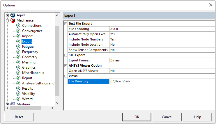
Export Views
A new Export category is available in the preferences dialog. The Views category provides the property File Directory. This property enables you to specify a default location to where you will export and/or import the graphical views that you have created, exported, or imported.
Want to learn more? If you are on Windows, go to the
documentation for this item by clicking
here
(Requires internet access and will open in a new browser window. Not for Linux platforms.)
Bearings Support Large Deflection
At 19.2, bearings support the Large Deflection property being set to On during Static and Transient Structural analyses.
Volume Result and Probe
Mechanical now provides a Volume result type as well as a Volume probe. This result and probe option supports body and element scoping and computes the total volume of the elements gathered through the scope.
Want to learn more? If you are on Windows, go to the
documentation for this item by clicking
here
(Requires internet access and will open in a new browser window. Not for Linux platforms.)

| Major Efforts | Physics Enhancements | Ease of Use Enhancements |
Major Efforts
Link Element definition
Line bodies may now be defined as links. Links have only X, Y & Z degrees of freedom (DOFs) and are often used in truss like structures.
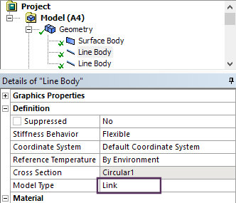
Link element definition
Want to learn more? If you are on Windows, go to the
documentation for this item by clicking
here
(Requires internet access and will open in a new browser window. Not for Linux platforms.)
Internal Pipe Contact
Line bodies defined as pipes can have internal contact to enable internal pipe contact.
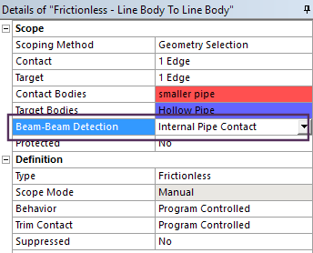 Contact setting for internal pipe contact |
 Beam element within a pipe element |
Want to learn more? If you are on Windows, go to the
documentation for this item by clicking
here
(Requires internet access and will open in a new browser window. Not for Linux platforms.)
New Static Acoustic System
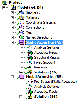 Prestressed Modal Acoustic analysis |
The new Static Acoustics analysis system on the project schematic page allows structural loads to be applied to models before acoustic simulations are carried out. 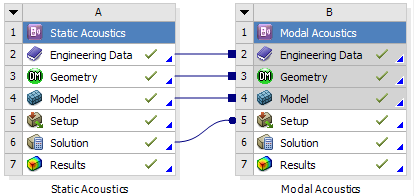 Prestressed modal acoustic model |
Want to learn more? If you are on Windows, go to the
documentation for this item by clicking
here
(Requires internet access and will open in a new browser window. Not for Linux platforms.)
Additional locations for Far Field Microphone results
Microphone Results now enable you to specify as many as nine microphone locations using the new Worksheet Definition Method option.
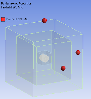 Far field microphone locations |
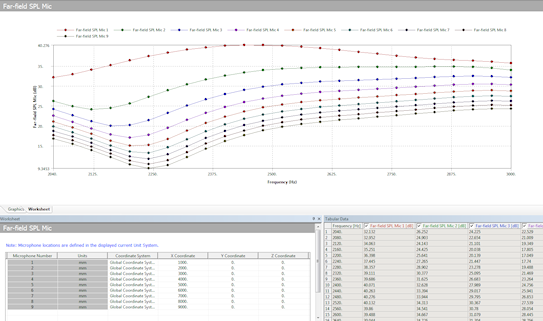 Far field microphone definition and response |
Want to learn more? If you are on Windows, go to the
documentation for this item by clicking
here
(Requires internet access and will open in a new browser window. Not for Linux platforms.)
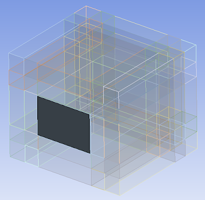
Diffuse Sound Field Transmission Loss
|
This is a new result type for Harmonic Acoustics analyses. It is used in combination with the Diffuse Sound Field excitation condition. It enables you to predict the transmission loss of the structural panel specified by the excitation. 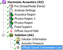 Diffuse sound result item |
 |
Want to learn more? If you are on Windows, go to the
documentation for this item by clicking
here
(Requires internet access and will open in a new browser window. Not for Linux platforms.)
SMART crack growth enhancements
|
The Smart Crack Growth object has a new property: Stop At Max Crack Extension. Using this property, you can specify the maximum distance for crack propagation. Once the maximum crack extension limit is reached, the application stops the solution process. In this instance, the solution is incomplete and the Solution folder will not be in solved state because the solution is not complete for all time points. If the maximum crack extension limit is not reached during solution, then the solution process completes normally. |
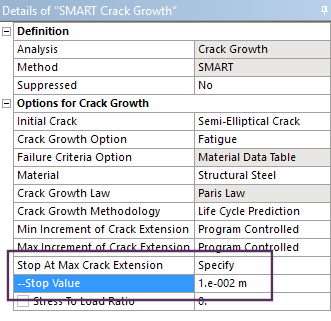 SMART fracture simulation - stop criteria definition |
Want to learn more? If you are on Windows, go to the
documentation for this item by clicking
here
(Requires internet access and will open in a new browser window. Not for Linux platforms.)
Temperature dependent Stress Life Fatigue
The Fatigue Tool now supports temperature dependent S-N Curves.
Note that the Engineering Data workspace material properties Alternating Stress Mean Stress and Alternating Stress R-Ratio are no longer available properties in the Life category. These have been replaced by the property S-N Curve, along with the new Mean Stress and R-Ratio Field Variables as well as Temperature.
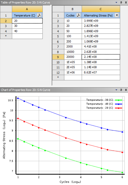
Temperature dependent S-N curve data
Want to learn more? If you are on Windows, go to the
documentation for this item by clicking
here
(Requires internet access and will open in a new browser window. Not for Linux platforms.)
Physics Enhancements
Pressure and link elements are imported
The External Model system now enables you to import link elements and pressure loads into Mechanical from Mechanical APDL CDB, ABAQUS Input, and Nastran Bulk Data files.
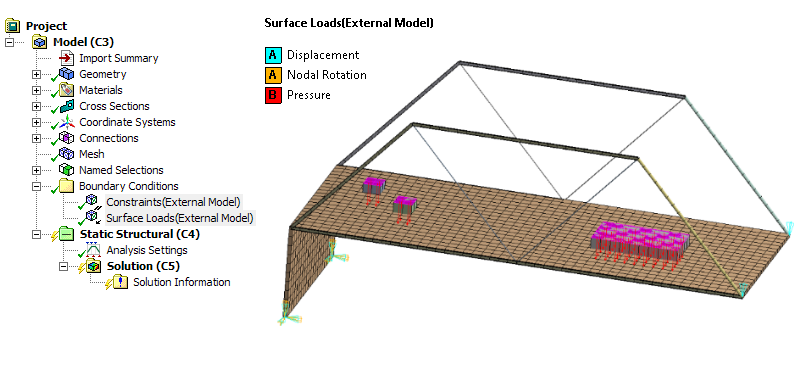
Imported surface loads
Want to learn more? If you are on Windows, go to the
documentation for these items by clicking
here for pressure and
here for link elements
(Requires internet access and will open in a new browser window. Not for Linux platforms.)
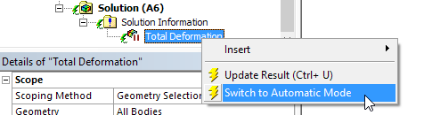
Result Plot Trackers During Solution
The Solution Information object provides Result Plot Tracker options that enable you to view result contours in real time as the solution progresses. Furthermore, you can add Result Plot Trackers at any point during the solution process.
In the previous release, this feature was only available for Topology Optimization analyses. Now, this feature has been expanded to include Static Structural, Transient Structural, Steady-State Thermal, Transient Thermal, and Explicit Dynamics analyses. New result options include Deformation, Stress, Strain, and Temperature.
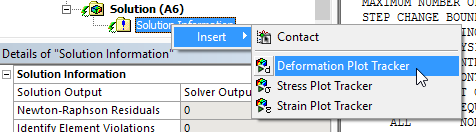
Result tracker update option
Want to learn more? If you are on Windows, go to the
documentation for this item by clicking
here
(Requires internet access and will open in a new browser window. Not for Linux platforms.)
Expanded scoping options for Response & Manufacturing Constraints
The Manufacturing Constraint condition now provides a Scope category of properties in the Details view for the Pull Out Direction, Cyclic, and Symmetry options of the Subtypes property. The scoping options enable you to scope these constraints to bodies and mesh elements, either geometry-based or Named Selections.
The Response Constraint condition now provides a Scope category of properties in the Details view. This category enables you to scope the Local von-Mises Stress Constraint to edges, faces, bodies, and mesh elements. In addition, you can scope the Displacement and Reaction Force constraints to vertices, edges, faces, bodies, and mesh nodes. For element and node scoping, you can specify one or more elements or nodes.
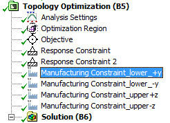 Multiple manufacturing constraints 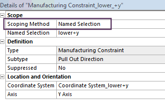 Named selection based constraints |
 |
Want to learn more? If you are on Windows, go to the
documentation for this item by clicking
here
(Requires internet access and will open in a new browser window. Not for Linux platforms.)
Ability to evaluate results at specific topological iterations
Result histories are now available for the Topology Density and Topology Elemental Density results. This means they can now be evaluated for specific iterations or animated over the solution.
The Iteration property enables you to specify an iteration number.
Animation of Topology Density iteration history
Want to learn more? If you are on Windows, go to the
documentation for these items by clicking
here for Topology Density and
here for Topology Elemental Density
(Requires internet access and will open in a new browser window. Not for Linux platforms.)
New product to model additive manufacturing print process simulation
|
ANSYS Additive Suite, an add-on product to Mechanical Enterprise level products, is now available to allow simulation of additive manufacturing processes. Transient thermal and a linked structural analysis are used with new AM Process tools built into Mechanical. Auto generated supports can be generated (if required). The process simulation allows simulation of thermal history, structural layer by layer simulation as well as build plate and support removal steps. A wizard is also available to guide users through the process of setting up an analysis. 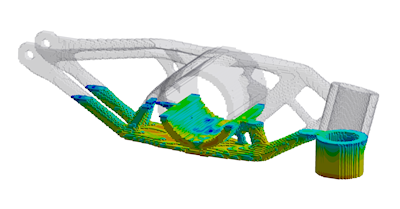 Half built AM part showing results as layers are added |
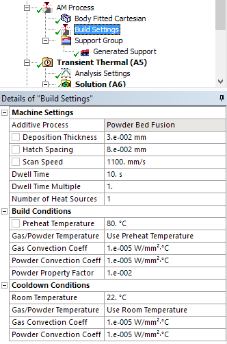 AM process settings |
Want to learn more? If you are on Windows, go to the
documentation for this item by clicking
here
(Requires internet access and will open in a new browser window. Not for Linux platforms.)
Ease of Use Enhancements
Granta Materials
Over 100 new materials from Granta have been included in 19.1.
A range of metals, plastics, woods and other materials have been added in the new "Granta Design Sample Materials" library.
You may also download additional nonlinear materials by visiting the link to Granta's website next to the material definitions in Engineering Data.
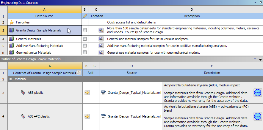
Materials from Granta
Want to learn more? If you are on Windows, go to the
documentation for this item by clicking
here
(Requires internet access and will open in a new browser window. Not for Linux platforms.)
Materials folder
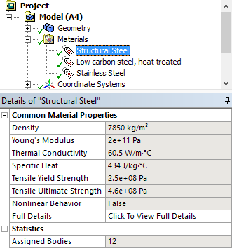 Materials folder with properties shown in details view |
Mechanical now provides a Materials object. This object contains all of the materials (in object form) available for your analysis. It is also used to insert and specify the following features:
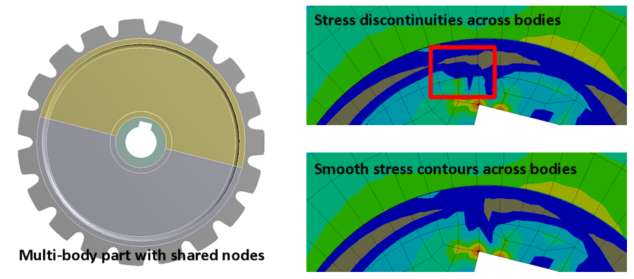
The new Material Assignment object enables you to assign materials to bodies and while doing so, share the same material ID across bodies in the solver input file. |
Consistent material ID's help with result averaging across multi-body parts
Want to learn more? If you are on Windows, go to the
documentation for this item by clicking
here
(Requires internet access and will open in a new browser window. Not for Linux platforms.)
Support Mirroring of geometry/mesh
The external model and model assembly import capability now supports mesh mirroring. Mirror plane location and the mirror plane can be specified.
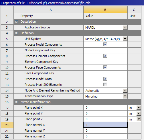 Mesh import mirroring option |
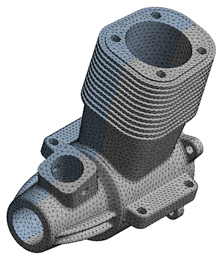 Imported mirrored mesh |
Want to learn more? If you are on Windows, go to the
documentation for this item by clicking
here
(Requires internet access and will open in a new browser window. Not for Linux platforms.)
Solution Statistics Page
The Solution Output property of the Solution Information object has a new option: Solution Statistics.
This option presents a quick summary of the solution process in the Worksheet. The summary includes solution and HPC metrics as well as recommendations to improve the solution time and performance.
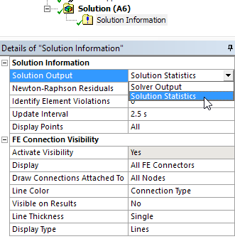 Solution Statistics option in Solution Information panel |
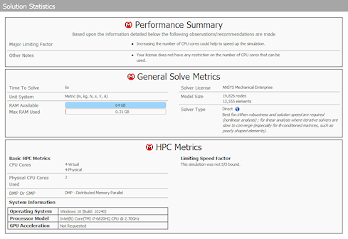 Sample Solution Statistics |
Want to learn more? If you are on Windows, go to the
documentation for this item by clicking
here
(Requires internet access and will open in a new browser window. Not for Linux platforms.)
MPEG, MP4 animation export
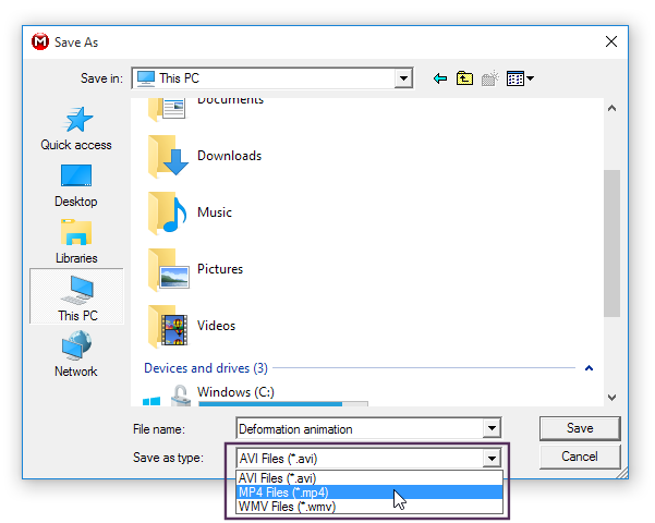 Animation export formats |
Animations can now be exported in multiple file formats. AVI, MP4 and WMV video file types can be created offering more flexibility. |
Ability to combine Workbench projects
Archived projects can now be imported into existing projects meaning projects can be combined.
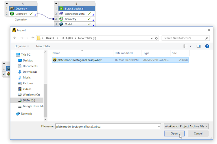
Project import dialog

| Major Efforts | Ease of Use Enhancements |
| Physics Enhancements | Advanced |
Major Efforts
S.M.A.R.T. Fracture
SMART (Separating, Morphing, Adaptive and Remeshing technology) is now natively available inside Mechanical.
Supports Mode I dominant crack propagation for static crack propagation based on failure criteria of Stress intensity factor or J-Integral.
Crack propagation based on Paris law defined in Engineering Data. Supports crack propagation of internally generated crack meshes, which includes Semi-elliptical and Arbitrary cracks as well as premeshed cracks.
SMART fracture simulation - exaggerated deformation (tet mesh on solid model)
Want to learn more? If you are on Windows, go to the
documentation for this item by clicking
here
(Requires internet access and will open in a new browser window. Not for Linux platforms.)
Acoustics
- Irregular Perfectly Matched Layers
- Power results (Transmission loss, absorption coefficient�)
- Frequency response results (pressure, spl, spla�)
- Element based force coupling between a Maxwell transient and a Harmonic (Transformer applications)
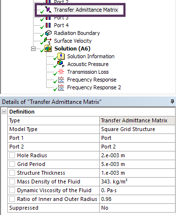
Transfer Admittance Matrix |
New transfer admittance matrix functionality boundary condition avoids need to mesh complex structures. Matrix can be parameterized and use either "Square Grid Structure" or "Hexagonal Grid Structure"
Applications in exhaust/muffler applications and anywhere mesh/grills are used. |


New controls to control radial axis bounds visibility controls for Far Field Polar plot. This helps to add clarity to plots covering larger ranges.
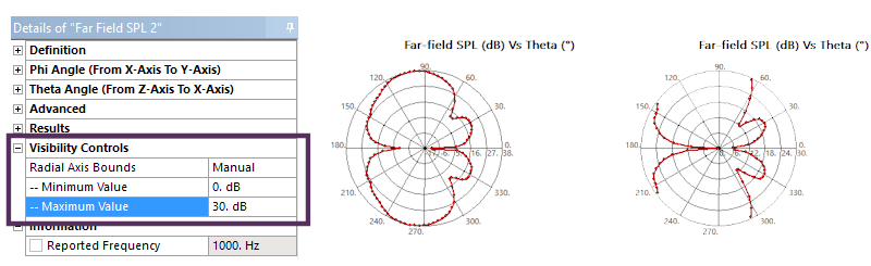
Full range vs. cropped to 30dB
Far field microphones allow you to plot acoustic quantities (pressure, SPL, SPLA, phase) function of the frequency at defined location outside the model mesh.
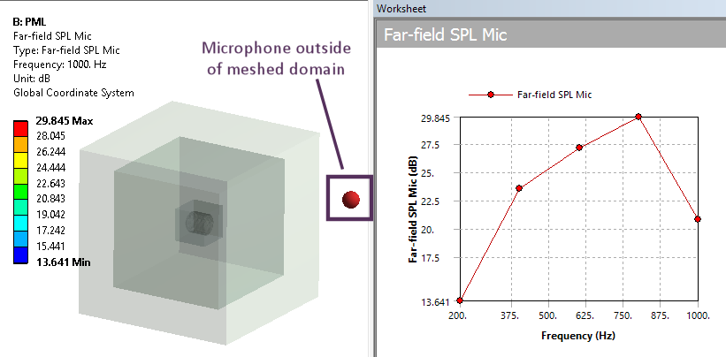
Micophone and SPL level outside of meshed domain
Want to learn more? If you are on Windows, go to the
documentation for these items by clicking
here for Transfer Admittance Matrix and
here for Far Field Microphones
(Requires internet access and will open in a new browser window. Not for Linux platforms.)
Topology Optimization
- Toplogy Optimization now supports RSM on both Windows and Linux clusters
- The Penalty factor (Penalty Parameter) is now available as part of the Analysis Settings
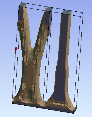
- Multiple manufacturing constraints can be applied to the model (ie. Pull-put direction and Symmetry)
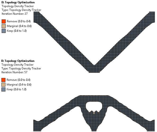
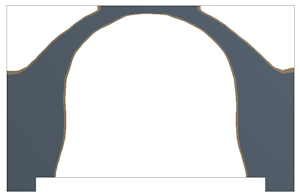
Minimizing deformation. Top: Vertical load with side constraints - Bottom: Vertical load with thermal load
Inertial loads now supported for optimization of load cases such as self weight. The following load types are supported:
|
Self weight topology optimization |
When a topology analysis has been carried out on a linked analysis, such as a prestressed modal, creating validation system now creates linked validation systems.
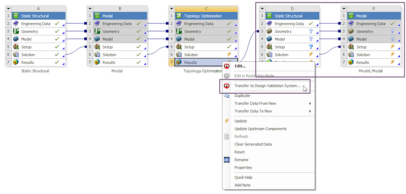
Transfer to Design Validation System creates linked systems
Want to learn more? If you are on Windows, go to the
documentation for this item by clicking
here
(Requires internet access and will open in a new browser window. Not for Linux platforms.)
Small sliding
|
Small sliding (now default for small deflection models) contact formulation results in more robust, faster and efficent solutions.
|
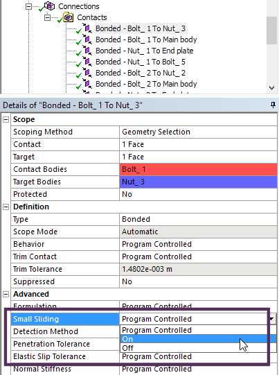
Details pane small sliding setting |
Want to learn more? If you are on Windows, go to the
documentation for this item by clicking
here
(Requires internet access and will open in a new browser window. Not for Linux platforms.)
Physics Enhancements
NLAD
NLAD (Non Linear ADaptivity) is now enabled for high order meshes. More analysis types can make use of this technique for models with larger deformations.
NLAD helps with models with extreme deformations
Want to learn more? If you are on Windows, go to the
documentation for this item by clicking
here
(Requires internet access and will open in a new browser window. Not for Linux platforms.)
External Model updates
External Model is now able to import a much greater set of models and boundary conditions from legacy ANSYS, Abaqus and Nastran.
Items supported include
- Boundary conditions
- Nodal loads
- Constraints
- Bolt pretension
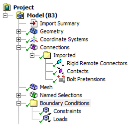 Imported loads and boudary conditions |
Nodal boundary conditions condtions can be imported from
|
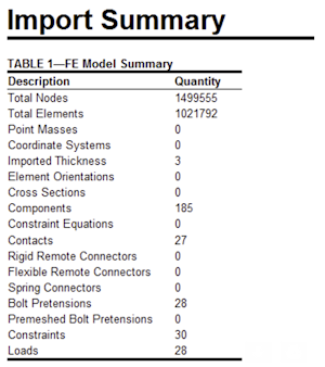 Import summary of translated objects |
Want to learn more? If you are on Windows, go to the
documentation for these items by clicking
here for Imported Load and Boundary Conditions and
here for a Summary of Translated Objects
(Requires internet access and will open in a new browser window. Not for Linux platforms.)
1 way FSI
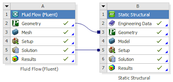
Fluent to Mechanical load transfer
A new Mechanical based mapping option is now available which vastly increases performance. In addition, duplication and copying of files between systems is eliminated.
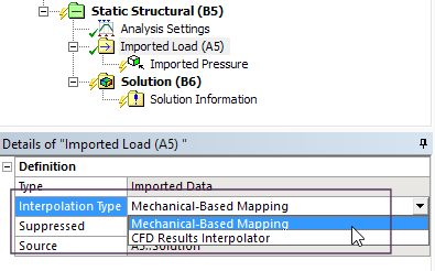
Mechanical-Based Mappping option
Want to learn more? If you are on Windows, go to the
documentation for this item by clicking
here
(Requires internet access and will open in a new browser window. Not for Linux platforms.)
Maxwell coupling
New ability to transfer EM forces from Maxwell to a frequency domain Harmonic Analysis. Maxwell Transient to Harmonic in addition to Maxwell Eddy Current to Harmonic.
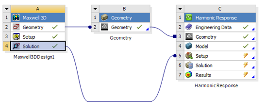
Transient Maxwell data transferred to Harmonic analysis
Ease of use Enhancements
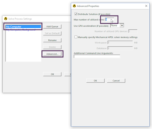
4 core HPC now enabled
|
Mechanical Pro, Mechanical Premium and Mechanical Enterprise (including multiphysics bundles) have access to upto 4 cores without the need for additional HPC licenses. To take advantage:
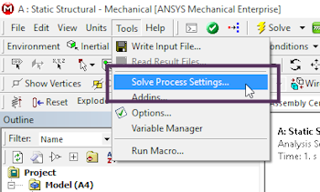
Setting output options |
Setting output options |
Average result quantities available
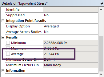
Average result value |
Two new result object properties are available: Average and Total. An Average value is provided for results when Minimum and Maximum values are listed. If the units of the result include Length, Area, Volume, Mass, Force, Moment, Energy, or Heat Rate, then the application provides the Total result value instead of the Average. These are parameterized quantities so can be used for driving optimization studies. |
Clipboard toolbar
The�Clipboard�toolbar is a selection feature that assists you to make, store and build up geometry or mesh selections.
Using the options of the�Clipboard�menu, you can create, change, add to, and overwrite your clipboard selections in order to temporarily save selection entities.
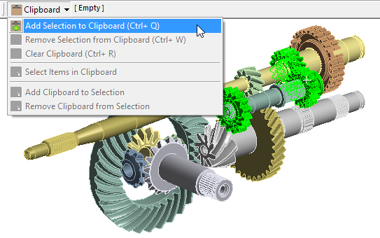
Adding 3 selected bodies to clipboard
Want to learn more? If you are on Windows, go to the
documentation for this item by clicking
here
(Requires internet access and will open in a new browser window. Not for Linux platforms.)
Material plots
|
New Material Plot feature under the geometry branch. Users can plot most material properties in the graphics window.
|
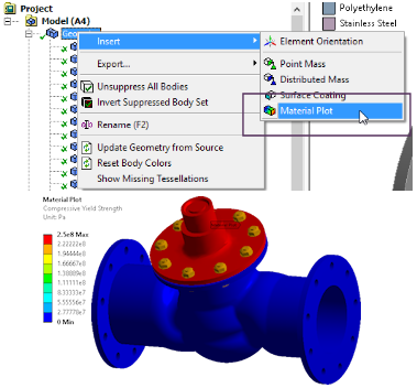 Compressive Yield Strength plot |
|
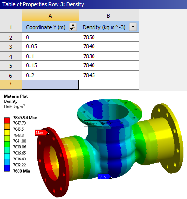 Spatially varying density plot |
Want to learn more? If you are on Windows, go to the
documentation for this item by clicking
here
(Requires internet access and will open in a new browser window. Not for Linux platforms.)
Local Minimums and Maximums
New right click option to create local mimumin and maximum values for result plots. The example below is showing local maximum von-Mises stress values.
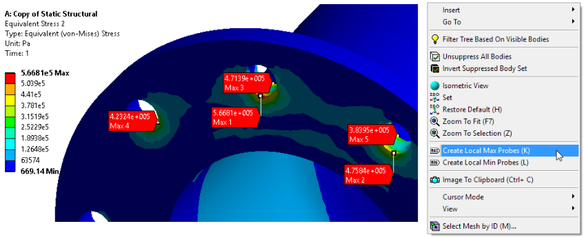
Local maximum von-Mises values
Want to learn more? If you are on Windows, go to the
documentation for this item by clicking
here
(Requires internet access and will open in a new browser window. Not for Linux platforms.)
Advanced
Birth and death
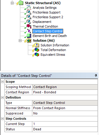
New objects for element and contact birth and death |
New controls for contact and element based birth and death now available in Mechanical. 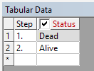
Tabular view of status Element and contact status can be controlled in a step-wise basis. Element status is now also reflected in post processing. 
Contact activation and element deactivation |
Want to learn more? If you are on Windows, go to the
documentation for this item by clicking
here
(Requires internet access and will open in a new browser window. Not for Linux platforms.)
Control result output
|
RST (result) file writing speed can be increased by only outputting displacement values. This results in faster solve times and smaller result files. Result items such as stress and strain can then be evaluated on demand from the stored displacement values. Note: This applies to linear static analysis only. 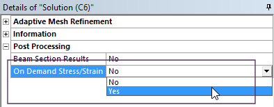
Setting for on-demand Stress/Strain |
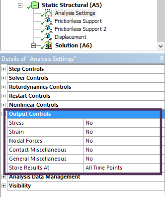
Setting output options |
Want to learn more? If you are on Windows, go to the
documentation for these items by clicking
here for Setting on-demand Stress/Strain and
here for Setting output options
(Requires internet access and will open in a new browser window. Not for Linux platforms.)
Result file postprocessing
|
A new result Scoping Method is available: Result File Item. In the previous release of Mechanical, this option was named Solver Component. You can scope results on solution generated Material IDs, Element Name IDs, and Element Type IDs, now you can also scope results to solver components. |
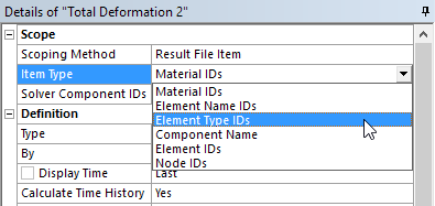
Result file scoping options |
Want to learn more? If you are on Windows, go to the
documentation for this item by clicking
here
(Requires internet access and will open in a new browser window. Not for Linux platforms.)